[1] "T1" "T2" "T3"Designing Experiments
This article is very much under construction, but check out
the old version of this chapter here
the packages {FielDHub} and {agricolae}
-
these publications:
Fundamental principles
In experimental design, three core principles are crucial: Replication, Randomization, and Blocking.
Replication (mandatory) involves repeating each treatment multiple times to distinguish real effects from random variations. For instance, in agricultural studies, a fertilizer treatment would be applied across several plots to accurately assess its impact.
Randomization (mandatory) ensures unbiased treatment assignment to experimental units, crucial for attributing outcome differences to the treatments rather than external factors. In clinical trials, this means randomly assigning patients to different treatment groups for comparability.
Blocking (optional) is used to control known sources of variability by grouping similar units. Treatments are randomized within these blocks, particularly effective in environments like field experiments where conditions like soil type can influence outcomes.
These principles - Replication for reliability, Randomization for unbiasedness, and Blocking for precision - are fundamental in designing robust experiments. A nice deep dive can be found in Casler (2015).
Possible Designs
In this section, we explore a variety of design models commonly employed in experimental life sciences, including fields such as agriculture, ecology, and biology. We will apply several functions provided by the {FielDHub} package, enabling us to generate and visualize exemplary layouts tailored to each design. It’s noteworthy to mention that {FielDHub}, despite being a relatively new tool, offers, in my opinion, superior capabilities for creating experimental designs compared to the more established {agricolae} package. Note that instead of real treatment levels, we will generate examplary levels like so:
CRD
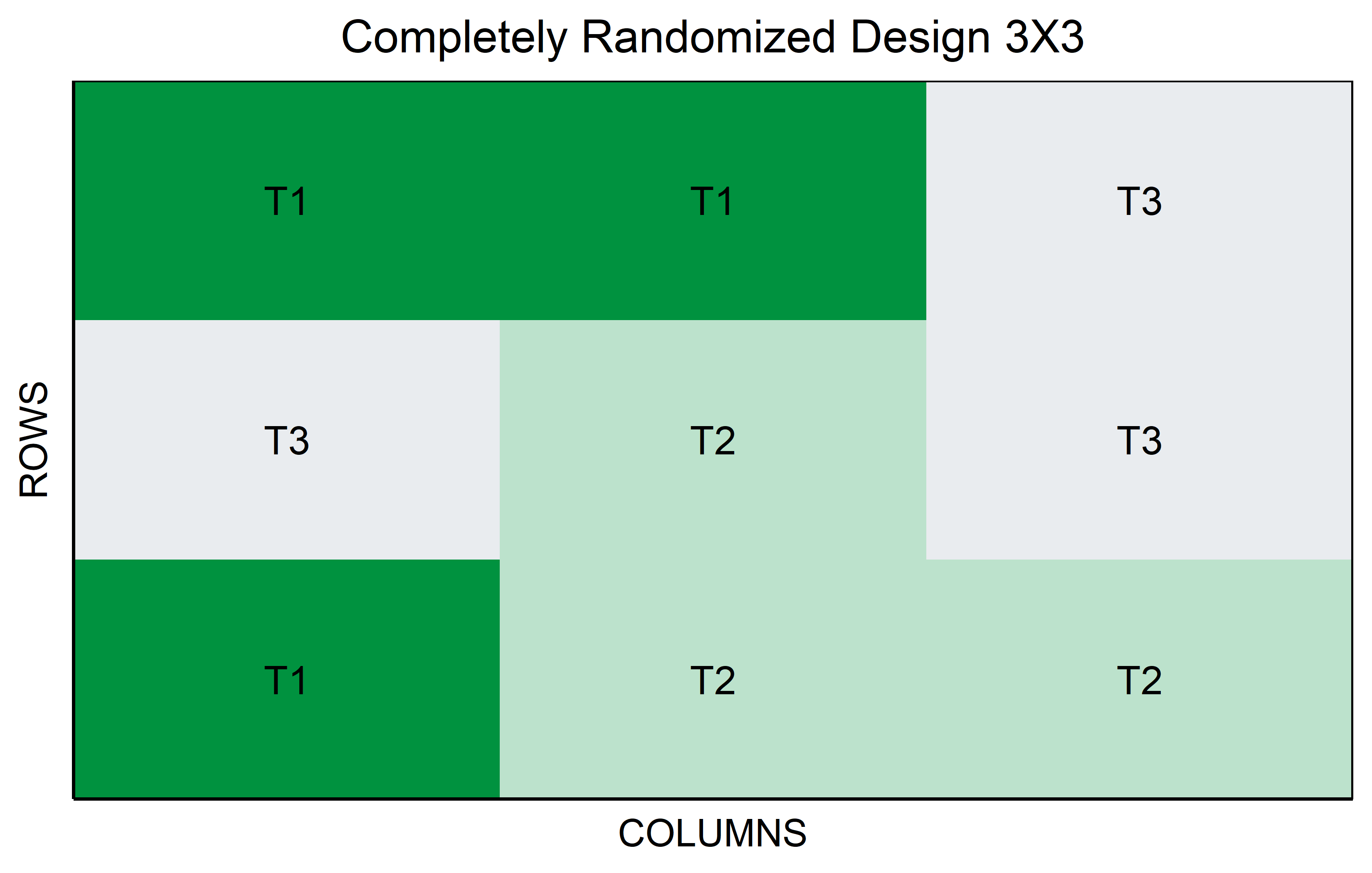
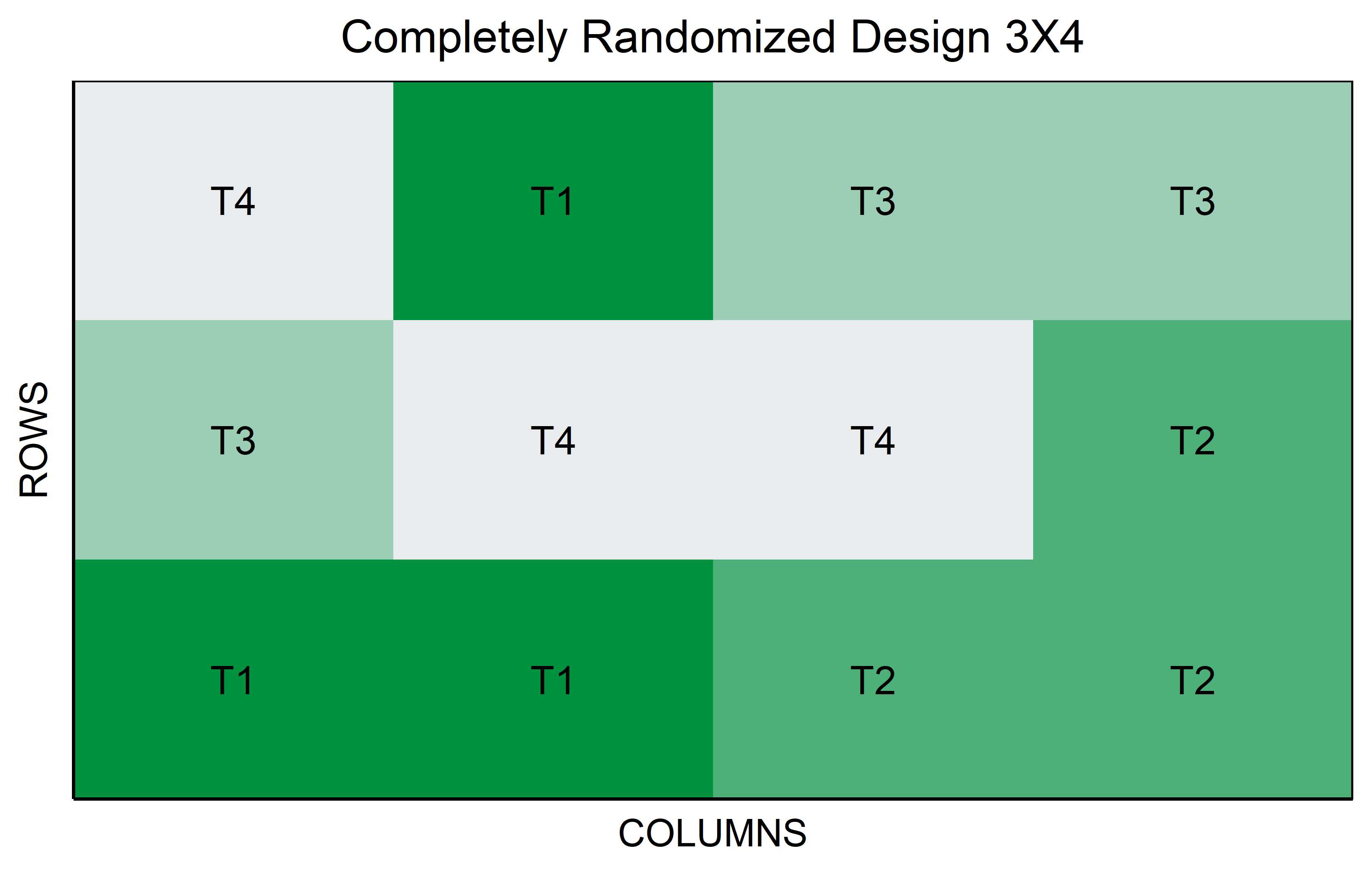
In a Completely Randomized Design (CRD), each experimental unit is assigned to a treatment completely at random, without any restrictions or grouping. This design is particularly useful when the experimental units are homogeneous or when the influence of external variables is minimal. In the context of genotypes, for example, each genotype (treatment level) is randomly allocated to the experimental units, such as plots or pots, ensuring that each treatment has an equal chance of being applied to any unit. Unlike designs with blocks or groups, the CRD does not account for potential variations among blocks or locations, making it a straightforward but powerful tool for experiments where external variability is low. This design’s simplicity makes it ideal for preliminary studies or scenarios where the primary goal is to assess the direct effects of treatments under controlled conditions.
can’t reproduce the colors?
You might be wondering why running the same code does not give you the same plots because your colors are different. This is because I actually changed the colors but hid the code that does so. If you want to see the entire code, go to the top right corner of this chapter, click on </> Code and then View Source.
RCBD
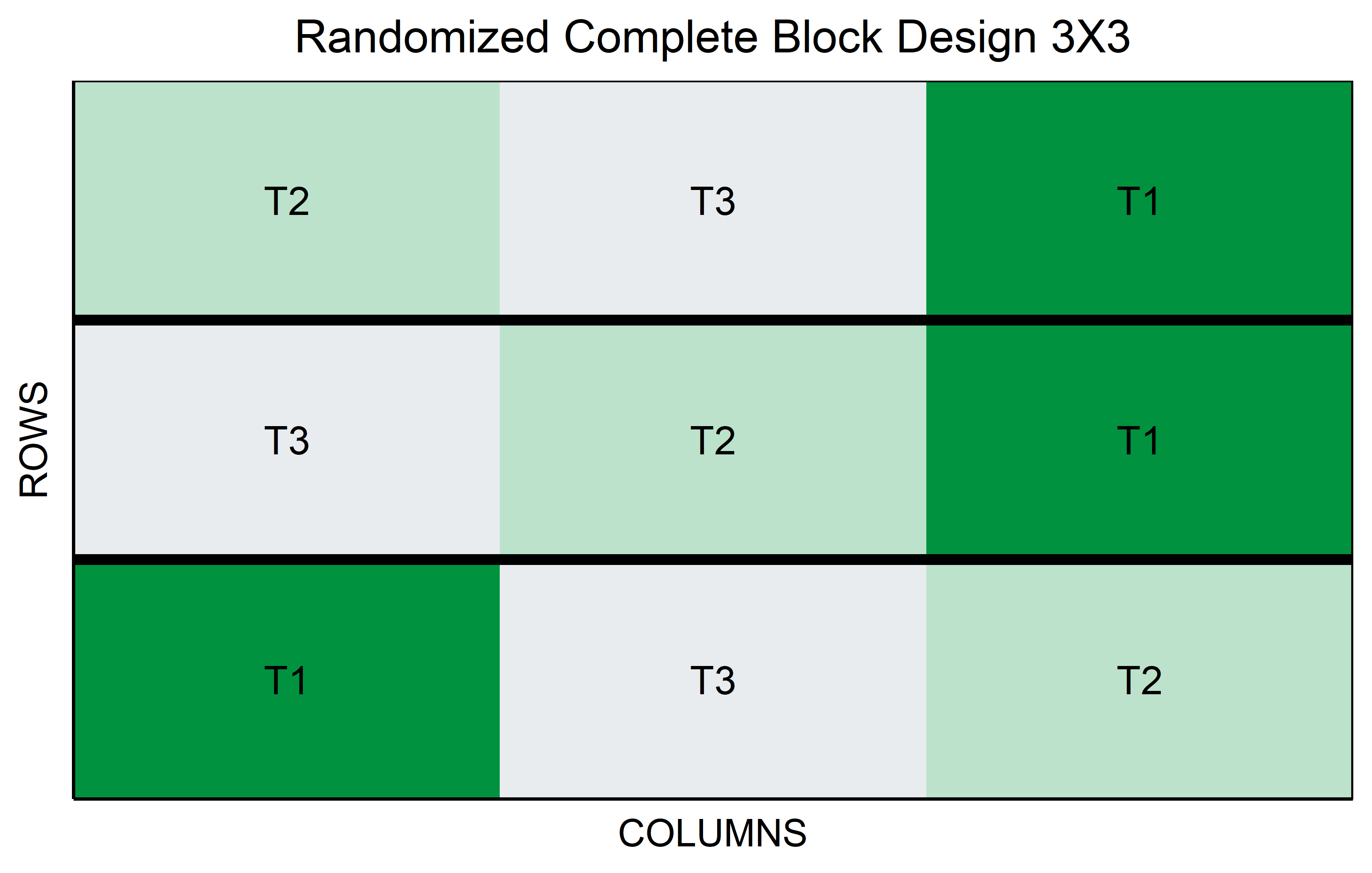
In a Randomized Complete Block Design (RCBD), treatments are randomly assigned within blocks, where each block is a grouping of experimental units that are similar in some way that is important to the experiment. This design is particularly effective in experiments where variability among the experimental units is expected, but can be grouped into relatively homogeneous blocks.
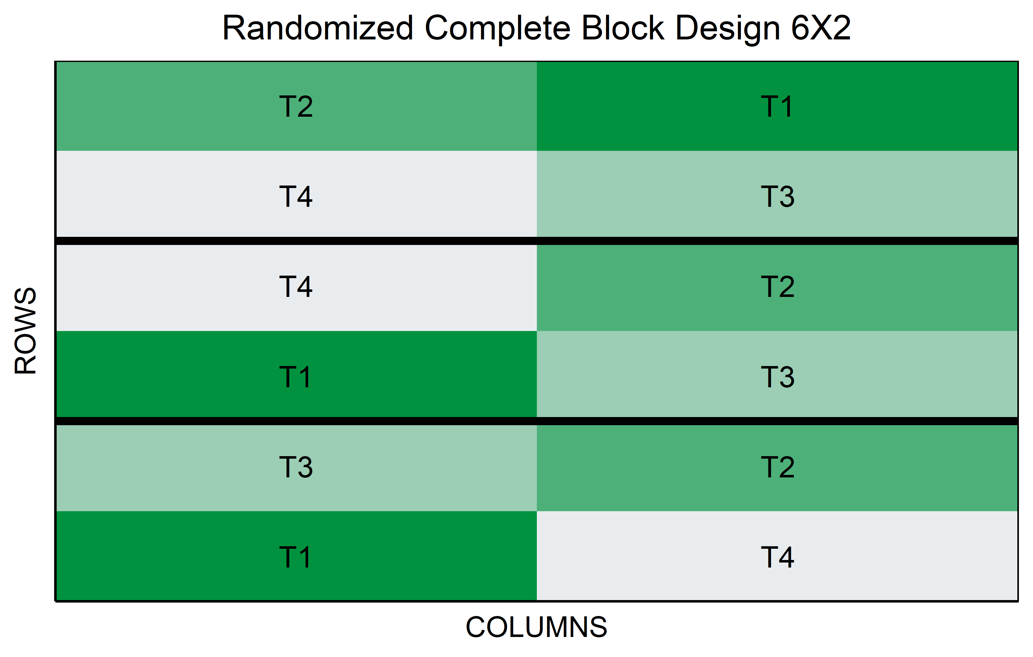
For instance, in agricultural experiments involving different genotypes, each block might represent a particular area of land with similar soil conditions. The key feature of an RCBD is that every treatment appears once in each block. This structure allows for the control of variation within blocks, making it easier to detect differences between treatments.
The RCBD is advantageous when external factors, such as environmental conditions or spatial effects, might influence the outcome. By comparing treatments within the same block, the RCBD controls for these external variations, providing a more accurate assessment of the treatment effects. This design is widely used in field experiments and other situations where controlling for external variability is crucial for obtaining reliable results.
Latin Square
In a Latin Square Design, the experiment is arranged in a square grid to control for two types of variability, such as different soil types (rows) and sunlight exposure (columns). Each treatment, like a specific genotype in an agricultural study, is assigned once in each row and column. This design efficiently manages two confounding variables with limited experimental units, ensuring that each treatment is evenly distributed across the varying conditions.
Code
out <- latin_square(
  t = 3,
  reps = 1,
  seed = 42
) %>% plot()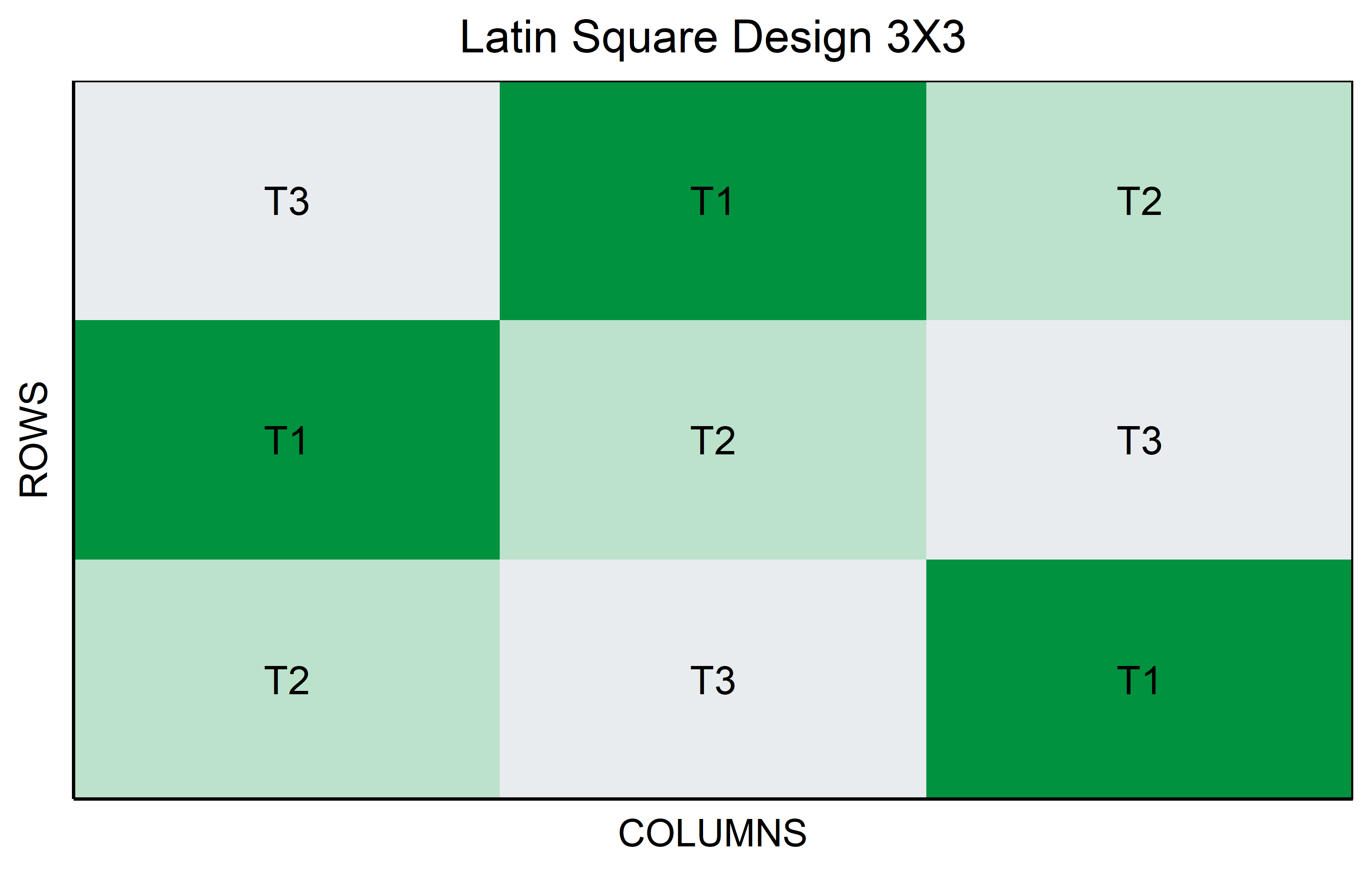
Code
out <- latin_square(
  t = 4,
  reps = 1,
  seed = 42
) %>% plot()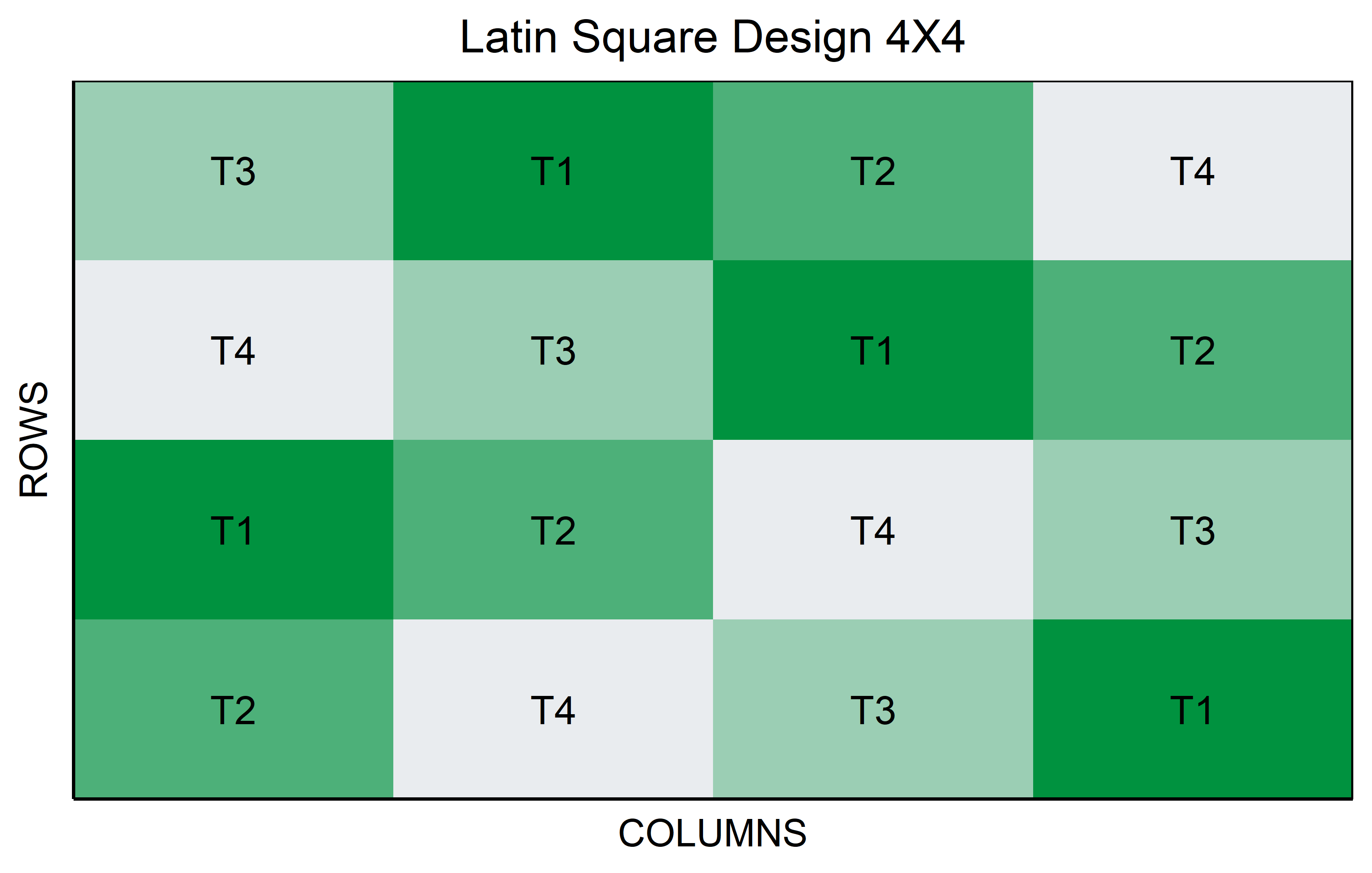
Augmented
In a non-resolvable1 Augmented Design, the treatment levels are categorized into two distinct groups. Within the realm of genotypes, these are identified as “lines” and “checks”. The lines represent the genotypes of interest, the primary focus of our study. On the other hand, checks are well-established genotypes that act as a standard reference, providing a reliable benchmark for comparing the performance of the lines. It’s important to note that the blocks are complete only in terms of the checks, meaning every check is present in each block. Conversely, the lines are introduced uniquely, appearing just once throughout the entire experiment. Through direct comparisons with the checks and indirect comparisons among the lines, valuable insights can be gleaned, making this design a practical choice in resource-limited situations.
Code
out <- RCBD_augmented(
  lines = 6,
  checks = 2,
  b = 3,
  seed = 42
) %>% plot()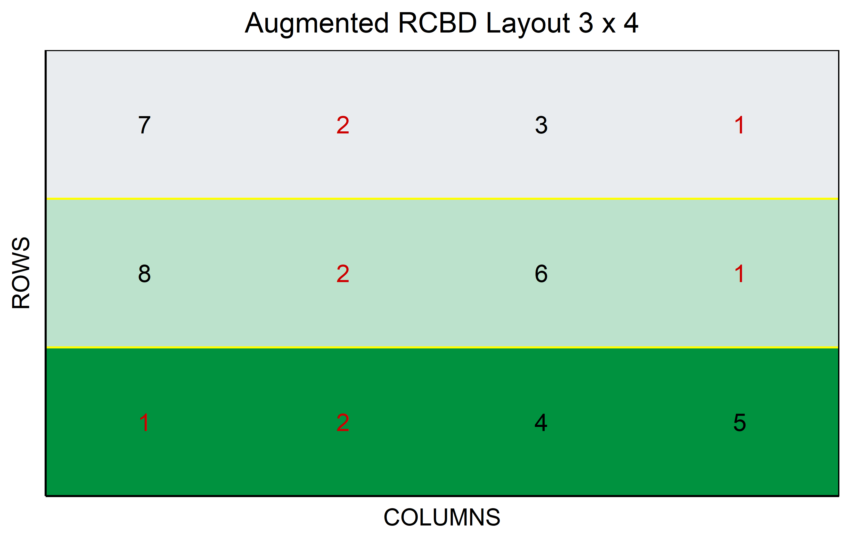
Code
out <- RCBD_augmented(
  lines = 30,
  checks = 3,
  b = 6,
  seed = 42
) %>% plot()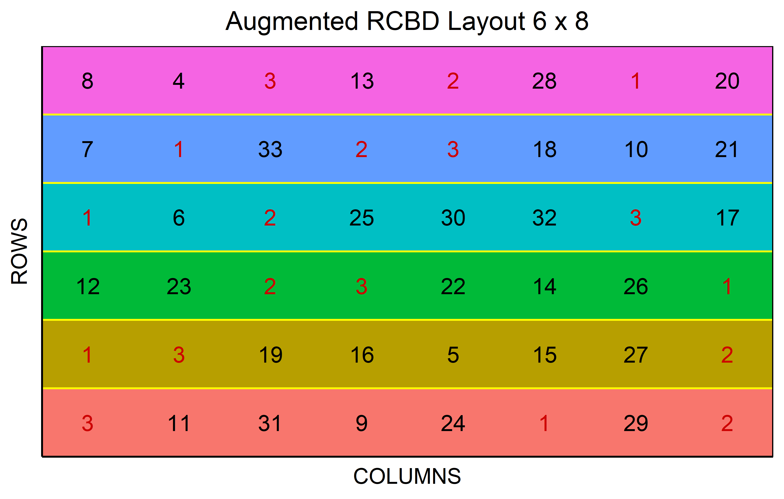
Alpha
An \(\alpha\)-design is an incomplete block design that is resolvable, meaning it is possible to group incomplete blocks into complete replicates. Thus, each treatment appears exactly once per replicate but obviously only in one of the incomplete blocks within each replicate, respectively. However, the assignment of treatments to the incomplete blocks is not random as it would be e.g. when simply taking an RCBD and separating the complete blocks further into incomplete blocks. Instead, the assignment is optimized so that any two treatments occur in the same incomplete-block in nearly equal frequency. In other words: The goal is to give any pair of treatments the same chance of appearing together in the same incomplete block to allow for a direct comparison. This design is defined by the formula \(v = sk\), where \(v\) is the number of treatments, \(s\) the number of blocks per replicate, and \(k\) the size of the incomplete blocks.
Code
out <- alpha_lattice(
  t = 9,
  k = 3,
  r = 3,
  seed = 42
) %>% plot()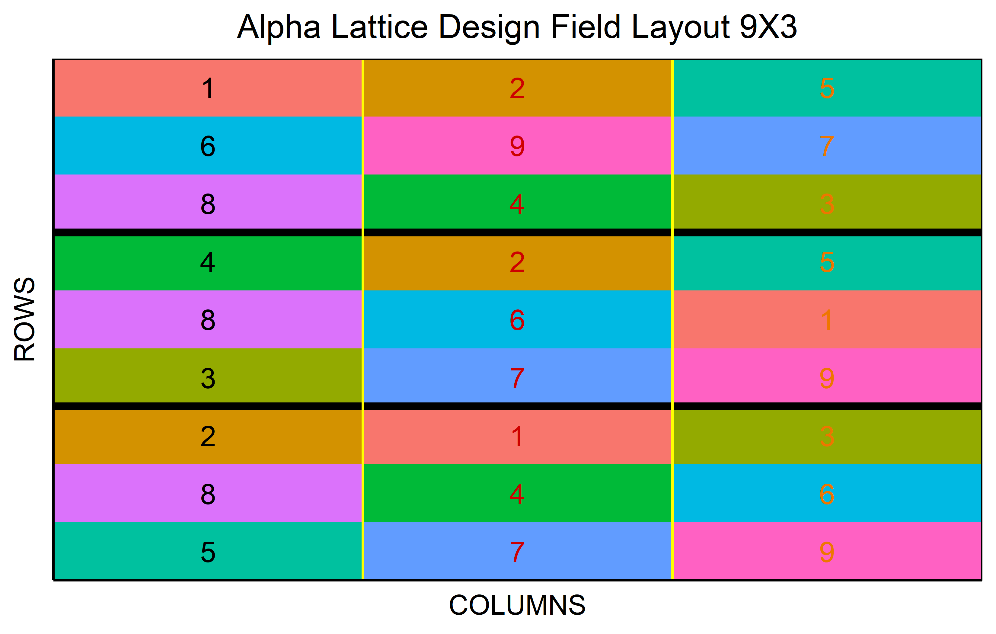
Code
out <- alpha_lattice(
  t = 15,
  k = 3,
  r = 3,
  seed = 42
) %>% plot()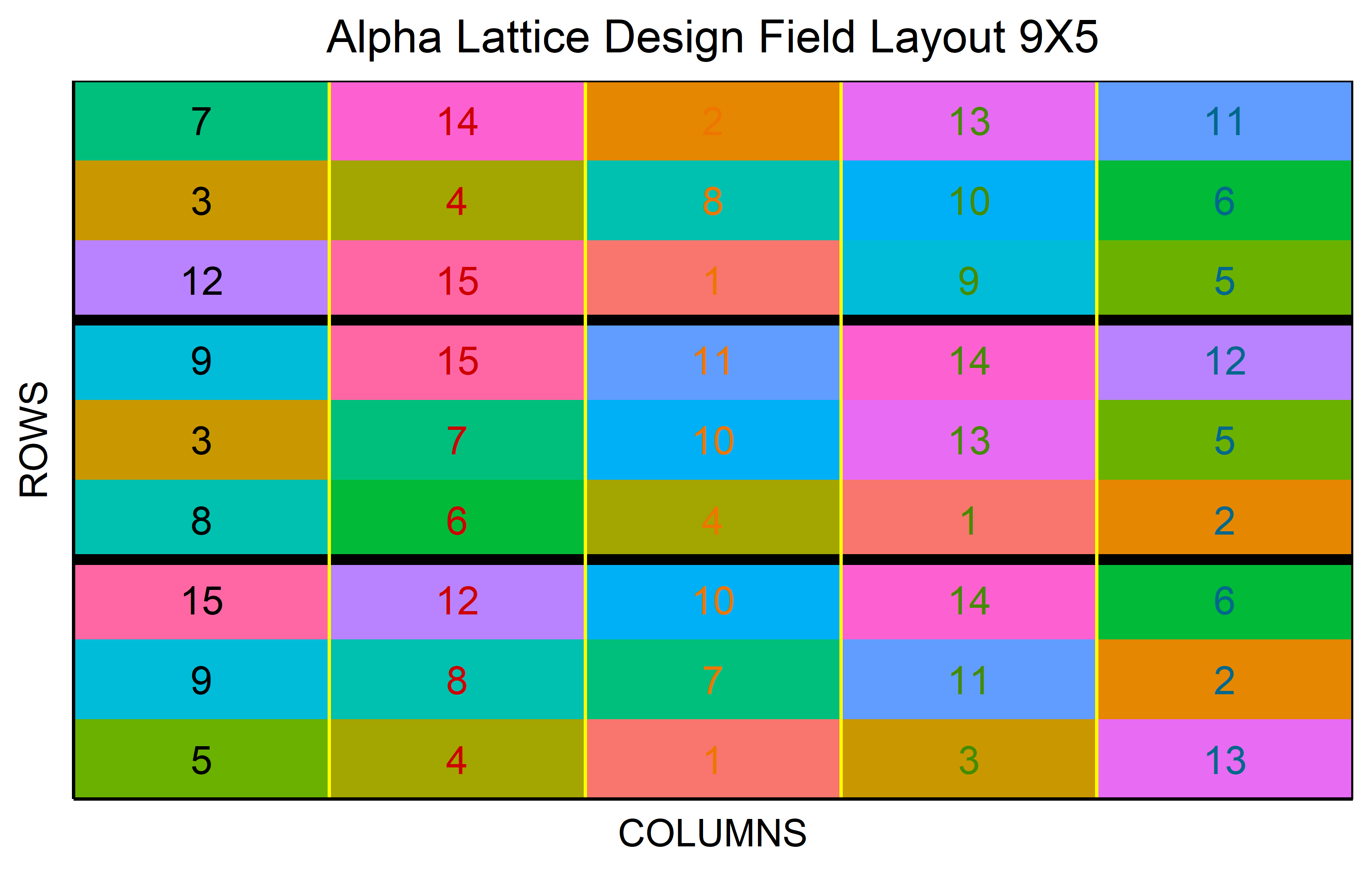
Row-Column
In a resolvable row-column design a complete replicate is divided into rows and columns. This creates a grid of incomplete blocks in both dimensions. The design’s resolvability lies in its ability to group these incomplete rows and columns back into complete replicates.
Code
out <- row_column(
  t = 6,
  nrows = 2,
  r = 3,
  seed = 42
) %>% plot()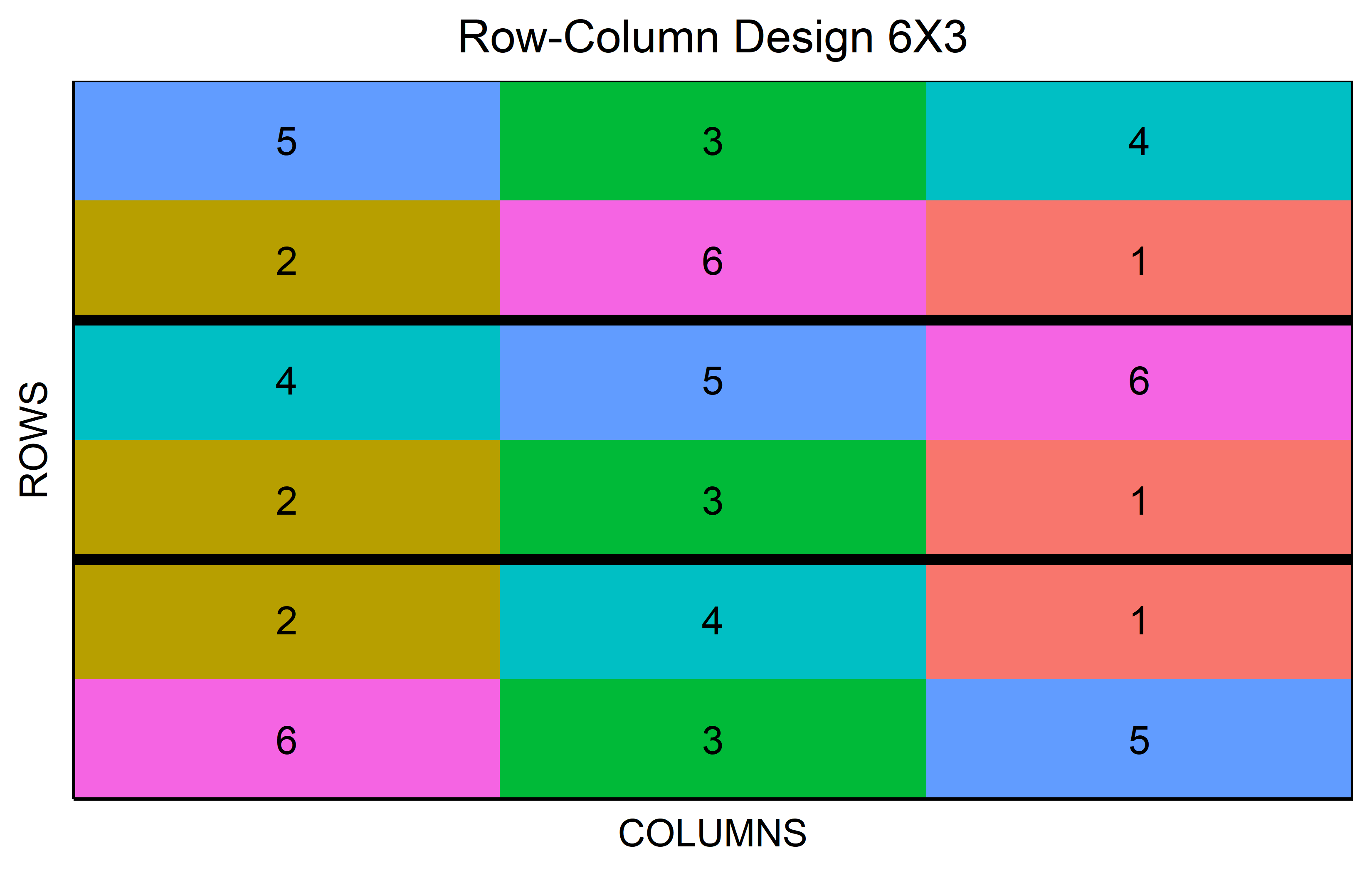
Code
out <- row_column(
  t = 12,
  nrows = 3,
  r = 3,
  seed = 42
) %>% plot()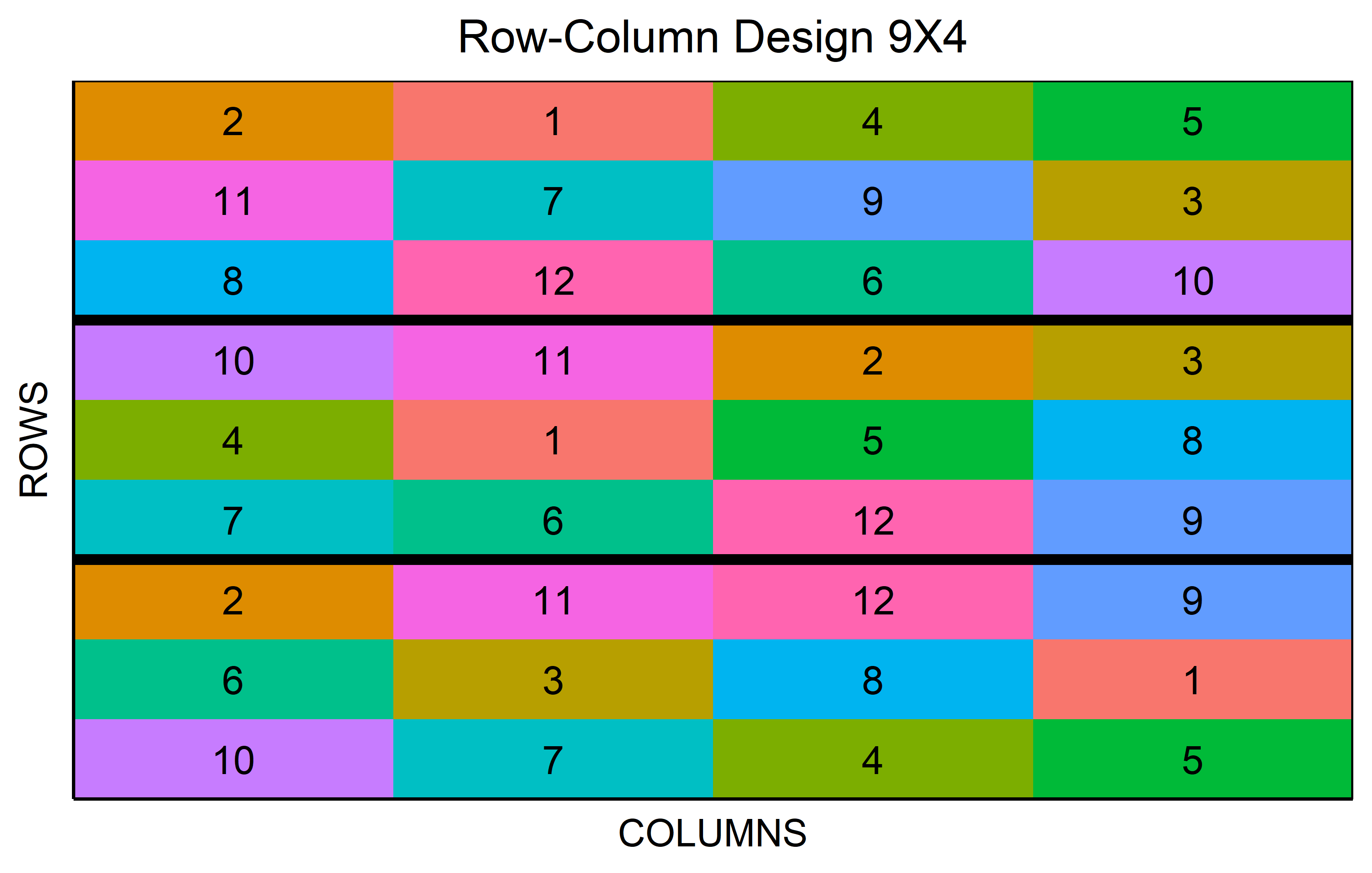
Split-plot
Split-plot designs are used in scenarios where two factors are involved, with one being easier or more cost-effective to randomize than the other.
Code
out <- split_plot(
  wp = paste0("A", 1:3),
  sp = paste0("B", 1:4),
  reps = 3,
  seed = 42
) %>% plot()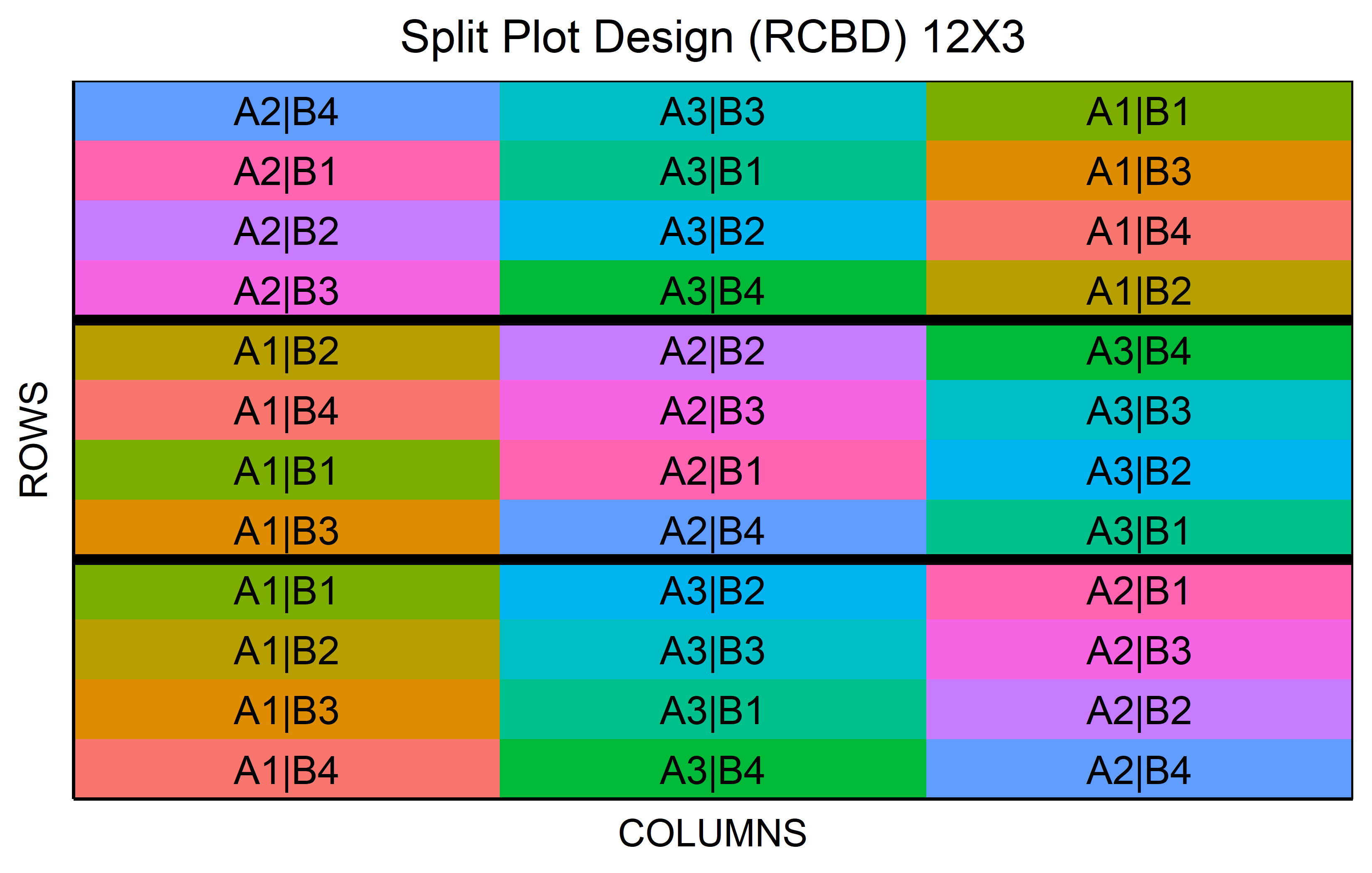
Code
out <- split_plot(
  wp = paste0("A", 1:2),
  sp = paste0("B", 1:5),
  reps = 2,
  seed = 42
) %>% plot()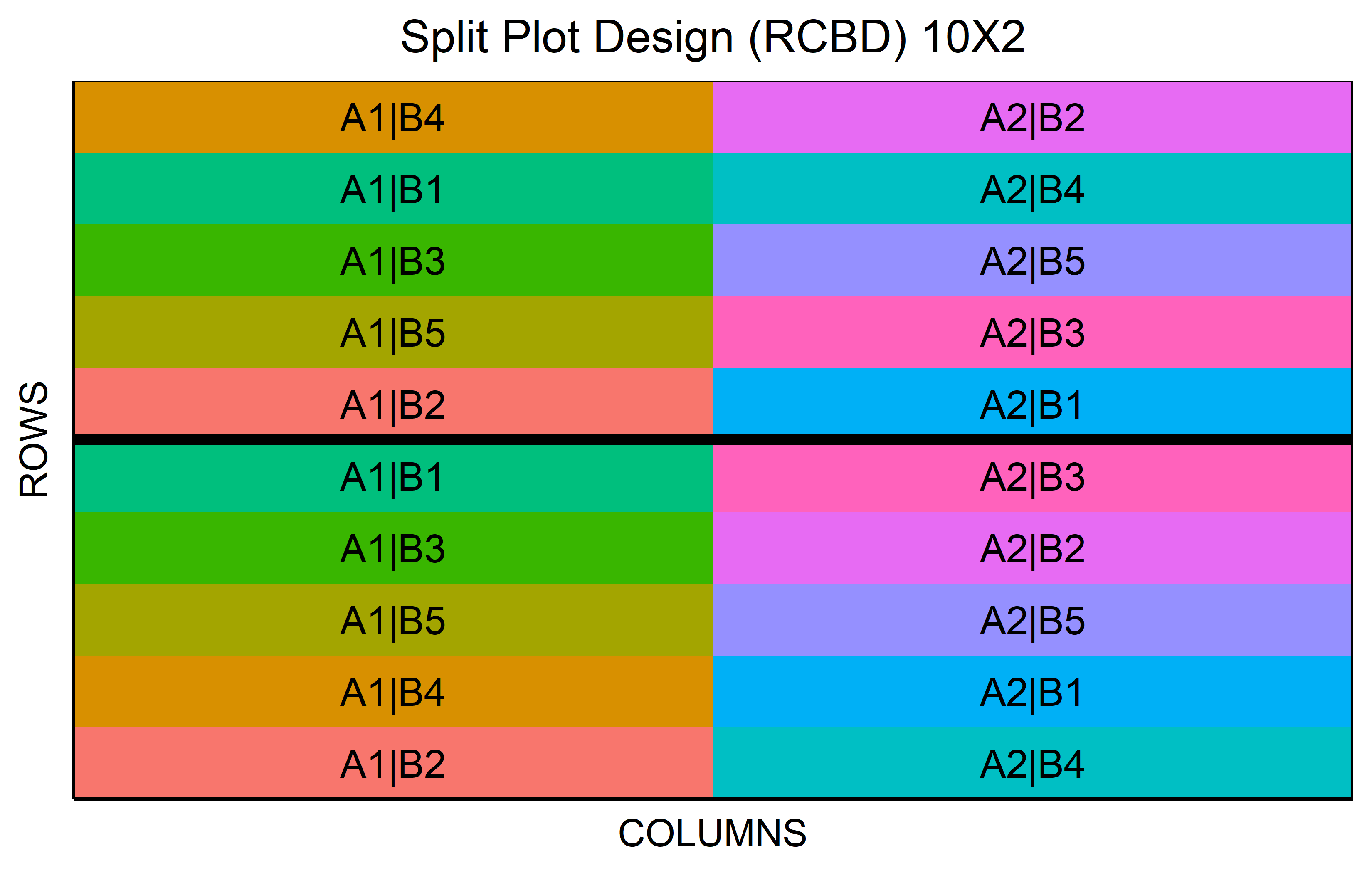
Sample Size
TODO
References
Casler, Michael D. 2015. “Fundamentals of Experimental Design: Guidelines for Designing Successful Experiments.” Agronomy Journal 107 (2): 692–705. https://doi.org/10.2134/agronj2013.0114.
Piepho, H. P., A. Büchse, and K. Emrich. 2003. “A Hitchhiker’s Guide to Mixed Models for Randomized Experiments.” Journal of Agronomy and Crop Science 189 (5): 310–22. https://doi.org/10.1046/j.1439-037X.2003.00049.x.
Piepho, H. P., A. Büchse, and C. Richter. 2004. “A Mixed Modelling Approach for Randomized Experiments with Repeated Measures.” Journal of Agronomy and Crop Science 190 (4): 230–47. https://doi.org/10.1111/j.1439-037X.2004.00097.x.
Piepho, Hans-Peter, Doreen Gabriel, Jens Hartung, Andreas Büchse, Meike Grosse, Sabine Kurz, Friedrich Laidig, et al. 2022. “One, Two, Three: Portable Sample Size in Agricultural Research.” The Journal of Agricultural Science 160 (6): 459–82. https://doi.org/10.1017/s0021859622000466.
Footnotes
The design is non-resolvable, since we cannot group incomplete blocks to form complete replicates.↩︎
Citation
BibTeX citation:
@online{schmidt2024,
  author = {Paul Schmidt},
  title = {Designing {Experiments}},
  date = {2024-03-28},
  url = {https://schmidtpaul.github.io/dsfair_quarto//ch/summaryarticles/designingexperiments.html},
  langid = {en}
}
For attribution, please cite this work as:
Paul Schmidt. 2024. “Designing Experiments.” March 28,
2024. https://schmidtpaul.github.io/dsfair_quarto//ch/summaryarticles/designingexperiments.html.