One-way augmented design
Data
This example is taken from Chapter “3.7 Analysis of a non-resolvable augmented design” of the course material “Mixed models for metric data (3402-451)” by Prof. Dr. Hans-Peter Piepho. It considers data published in Petersen (1994) from a yield trial laid out as an augmented design. The genotypes (gen) include 3 standards (st, ci, wa) and 30 new cultivars of interest. The trial was laid out in 6 blocks (block). The 3 standards are tested in each block, while each entry is tested in only one of the blocks. Therefore, the blocks are “incomplete blocks”.
Import
# data is available online:
path <- "https://raw.githubusercontent.com/SchmidtPaul/dsfair_quarto/master/data/Petersen1994.csv"
dat <- read_csv(path) # use path from above
dat# A tibble: 48 × 5
gen yield block row col
<chr> <dbl> <chr> <dbl> <dbl>
1 st 2972 I 1 1
2 14 2405 I 2 1
3 26 2855 I 3 1
4 ci 2592 I 4 1
5 17 2572 I 5 1
6 wa 2608 I 6 1
7 22 2705 I 7 1
8 13 2391 I 8 1
9 st 3122 II 1 2
10 ci 3023 II 2 2
# ℹ 38 more rowsFormat
Before anything, the columns gen and block should be encoded as factors, since R by default encoded them as character.
Explore
We make use of dlookr::describe() to conveniently obtain descriptive summary tables. Here, we get can summarize per block and per cultivar.
dat %>%
  group_by(gen) %>%
  dlookr::describe(yield) %>%
  select(2:sd) %>%
  arrange(desc(n), desc(mean))
# A tibble: 33 × 5
gen n na mean sd
<fct> <int> <int> <dbl> <dbl>
1 st 6 0 2759. 832.
2 ci 6 0 2726. 711.
3 wa 6 0 2678. 615.
4 19 1 0 3643 NA
5 11 1 0 3380 NA
6 07 1 0 3265 NA
7 03 1 0 3055 NA
8 04 1 0 3018 NA
9 01 1 0 3013 NA
10 30 1 0 2955 NA
# ℹ 23 more rowsdat %>%
group_by(block) %>%
dlookr::describe(yield) %>%
select(2:sd) %>%
arrange(desc(mean))# A tibble: 6 × 5
block n na mean sd
<fct> <int> <int> <dbl> <dbl>
1 VI 8 0 3205. 417.
2 II 8 0 2864. 258.
3 IV 8 0 2797. 445.
4 I 8 0 2638. 202.
5 III 8 0 2567. 440.
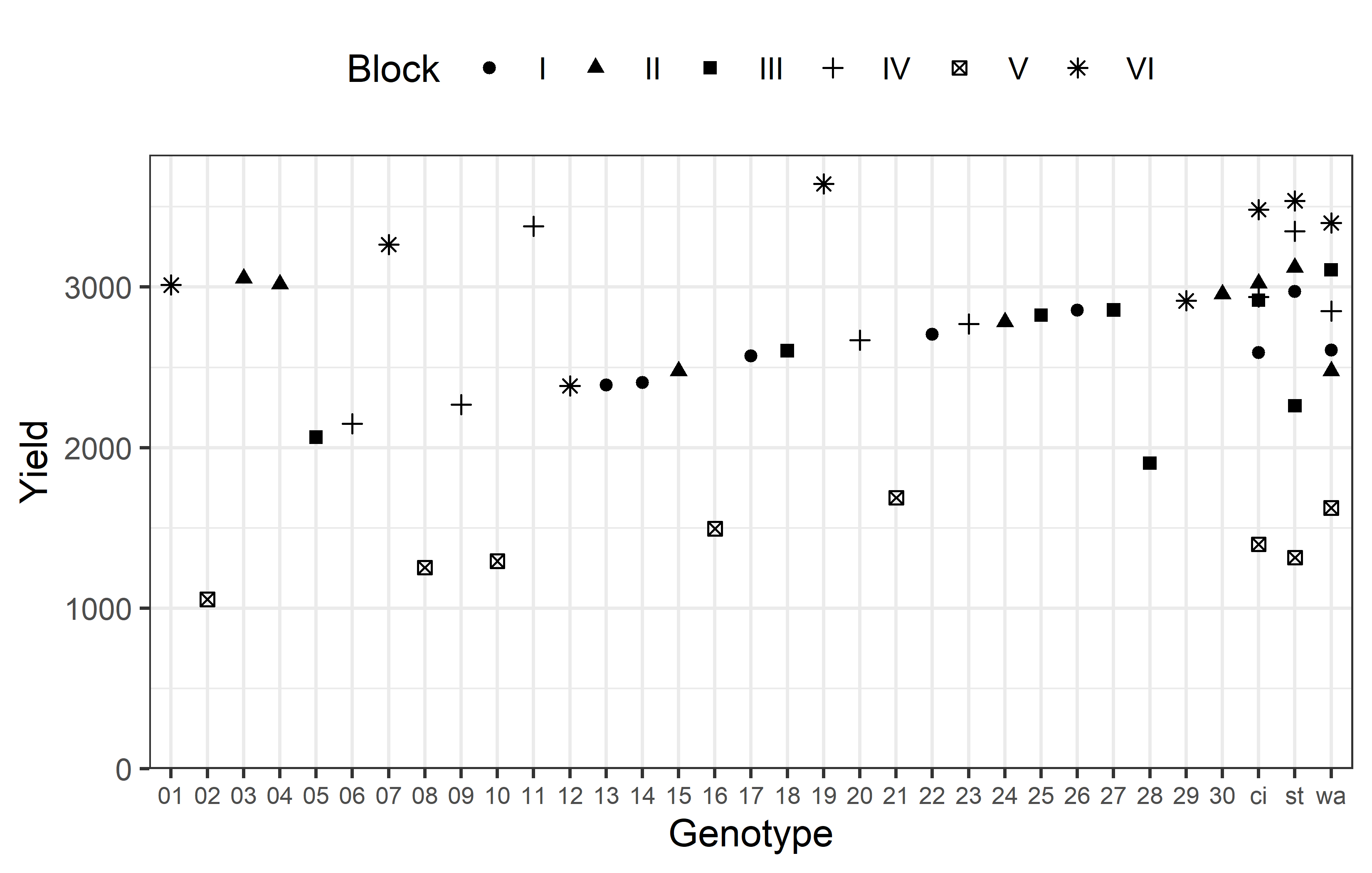
6 V 8 0 1390. 207.Additionally, we can decide to plot our data. Note that we here define custom colors for the genotypes, where all unreplicated entries get a shade of green and all replicated checks get a shade of red.
greens30 <- colorRampPalette(c("#bce2cc", "#00923f"))(30)
oranges3 <- colorRampPalette(c("#e4572e", "#ad0000"))(3)
gen_cols <- set_names(c(greens30, oranges3), nm = levels(dat$gen))
Code
ggplot(data = dat) +
  aes(
    y = yield,
    x = gen,
    shape = block
  ) +
  geom_point() +
    scale_x_discrete(
    name = "Genotype"
  ) +
  scale_y_continuous(
    name = "Yield",
    limits = c(0, NA),
    expand = expansion(mult = c(0, 0.05))
  ) +
  scale_color_manual(
    guide = "none",
    values = gen_cols
  ) +
  scale_shape_discrete(
    name = "Block"
  ) +
  guides(shape = guide_legend(nrow = 1)) +
  theme_bw() +
  theme(
    legend.position = "top",
    axis.text.x = element_text(size = 7)
  )
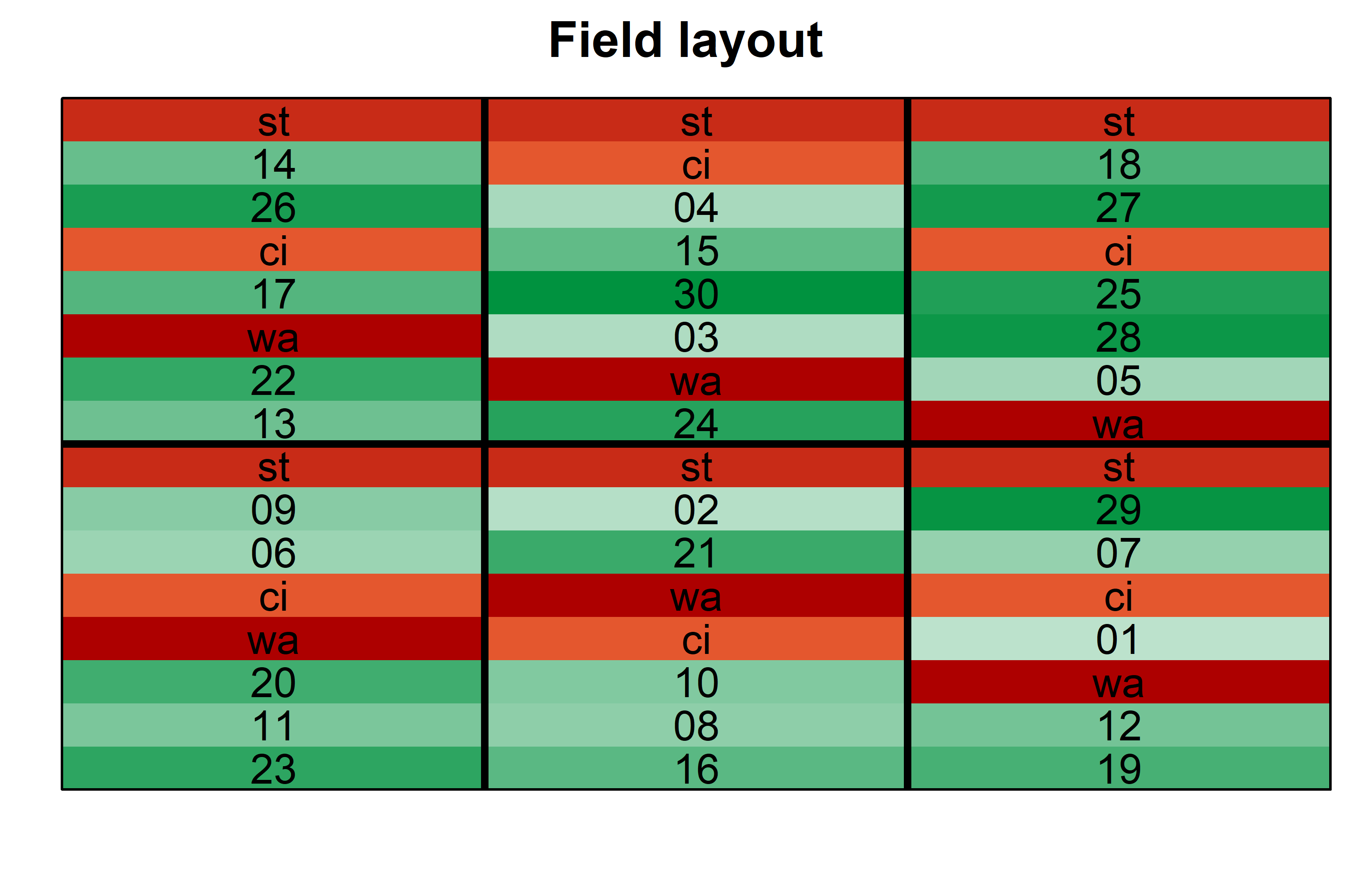
Finally, since this is an experiment that was laid with a certain experimental design (= a non-resolvable augmented design) - it makes sense to also get a field plan. This can be done via desplot() from {desplot}.
Code
desplot(
  data = dat,
  flip = TRUE, # row 1 on top, not on bottom
  form = gen ~ col + row, # fill color per cultivar
  col.regions = gen_cols, # custom fill colors
  out1 = block, # line between blocks
  text = gen, # cultivar names per plot
  cex = 1, # cultviar names: font size
  shorten = FALSE, # cultivar names: don't abbreviate
  main = "Field layout", # plot title
  show.key = FALSE # hide legend
) 
Model
Finally, we can decide to fit a linear model with yield as the response variable and gen as fixed effects, since our goal is to compare them to each other. Since the trial was laid out in blocks, we also need block effects in the model, but these can be taken either as a fixed or as random effects. Since our goal is to compare genotypes, we will determine which of the two models we prefer by comparing the average standard error of a difference (s.e.d.) for the comparisons between adjusted genotype means - the lower the s.e.d. the better.
# blocks as random (linear mixed model)
mod_rb <- lmer(yield ~ gen + (1 | block),
               data = dat)

mod_rb %>%
  emmeans(pairwise ~ "gen",
          adjust = "tukey",
          lmer.df = "kenward-roger") %>%
  pluck("contrasts") %>% # extract diffs
  as_tibble() %>% # format to table
  pull("SE") %>% # extract s.e.d. column
  mean() # get arithmetic mean
[1] 462.0431As a result, we find that the model with fixed block effects has the slightly smaller s.e.d. and is therefore more precise in terms of comparing genotypes.
It would be at this moment (i.e. after fitting the model and before running the ANOVA), that you should check whether the model assumptions are met. Find out more in the summary article “Model Diagnostics”
ANOVA
Based on our model, we can then conduct an ANOVA:
ANOVA <- car::Anova(mod_fb, type = "III")
ANOVA
Anova Table (Type III tests)
Response: yield
Sum Sq Df F value Pr(>F)
(Intercept) 3073607 1 33.738 0.0001710 ***
gen 4095905 32 1.405 0.2930113
block 6968486 5 15.298 0.0002082 ***
Residuals 911027 10
---
Signif. codes: 0 '***' 0.001 '**' 0.01 '*' 0.05 '.' 0.1 ' ' 1Accordingly, the ANOVA’s F-test found the cultivar effects to be statistically significant (p = 0.293). Additionally, the block effects are also statistically significant (p < .001***), but this is only of secondary concern for us.
Mean comparison
Besides an ANOVA, one may also want to compare adjusted yield means between cultivars via post hoc tests (t-test, Tukey test etc.).
mean_comp <- mod_fb %>%
  emmeans(specs = ~ gen) %>% # adj. mean per genotype
  cld(adjust = "Tukey", Letters = letters) # compact letter display (CLD)

mean_comp
gen emmean SE df lower.CL upper.CL .group
12 1632 341 10 164 3100 a
06 1823 341 10 355 3291 a
28 1862 341 10 394 3330 a
09 1943 341 10 475 3411 a
05 2024 341 10 556 3492 a
29 2162 341 10 694 3630 a
01 2260 341 10 792 3728 a
15 2324 341 10 856 3792 a
02 2330 341 10 862 3798 a
20 2345 341 10 877 3813 a
13 2388 341 10 920 3856 a
14 2402 341 10 934 3870 a
23 2445 341 10 977 3913 a
07 2512 341 10 1044 3980 a
08 2528 341 10 1060 3996 a
18 2562 341 10 1094 4030 a
10 2568 341 10 1100 4036 a
17 2569 341 10 1101 4037 a
24 2630 341 10 1162 4098 a
wa 2678 123 10 2148 3208 a
22 2702 341 10 1234 4170 a
ci 2726 123 10 2195 3256 a
st 2759 123 10 2229 3289 a
16 2770 341 10 1302 4238 a
25 2784 341 10 1316 4252 a
30 2802 341 10 1334 4270 a
27 2816 341 10 1348 4284 a
26 2852 341 10 1384 4320 a
04 2865 341 10 1397 4333 a
19 2890 341 10 1422 4358 a
03 2902 341 10 1434 4370 a
21 2963 341 10 1495 4431 a
11 3055 341 10 1587 4523 a
Results are averaged over the levels of: block
Confidence level used: 0.95
Conf-level adjustment: sidak method for 33 estimates
P value adjustment: tukey method for comparing a family of 33 estimates
significance level used: alpha = 0.05
NOTE: If two or more means share the same grouping symbol,
then we cannot show them to be different.
But we also did not show them to be the same. It can be seen that while some genotypes have a higher yield than others, no differences are found to be statistically significant here. Accordingly, notice that e.g. for gen 11, which is the genotype with the highest adjusted yield mean (=3055), its lower confidence limit (=1587) includes gen 12, which is the genotype with the lowest adjusted yield mean (=1632).
Note that if you would like to see the underlying individual contrasts/differences between adjusted means, simply add details = TRUE to the cld() statement. Furthermore, check out the Summary Article “Compact Letter Display”.
Finally, we can create a plot that displays both the raw data and the results, i.e. the comparisons of the adjusted means that are based on the linear model.
Code
# reorder genotype factor levels according to adjusted mean
my_caption <- "Dots represent raw data. Red diamonds and error bars represent adjusted means with 95% confidence limits per cultivar. Means followed by a common letter are not significantly different according to the Tukey-test."

ggplot() +
  # green/red dots representing the raw data
  geom_point(
    data = dat,
    aes(y = yield, x = gen, color = gen)
  ) +
  # red diamonds representing the adjusted means
  geom_point(
    data = mean_comp,
    aes(y = emmean, x = gen),
    shape = 18,
    color = "red",
    position = position_nudge(x = 0.2)
  ) +
  # red error bars representing the confidence limits of the adjusted means
  geom_errorbar(
    data = mean_comp,
    aes(ymin = lower.CL, ymax = upper.CL, x = gen),
    color = "red",
    width = 0.1,
    position = position_nudge(x = 0.2)
  ) +
  # red letters
  geom_text(
    data = mean_comp,
    aes(y = upper.CL, x = gen, label = str_trim(.group)),
    color = "red",
    vjust = -0.2,
    position = position_nudge(x = 0.2)
  ) +
  scale_color_manual(
    guide = "none",
    values = gen_cols
  ) +
  scale_x_discrete(
    name = "Cultivar",
    limits = as.character(mean_comp$gen)
  ) +
  scale_y_continuous(
    name = "Yield",
    limits = c(0, NA),
    expand = expansion(mult = c(0, 0.1))
  ) +
  labs(caption = my_caption) +
  theme_classic() +
  theme(plot.caption = element_textbox_simple(margin = margin(t = 5)),
        plot.caption.position = "plot",
        axis.text.x = element_text(size = 7))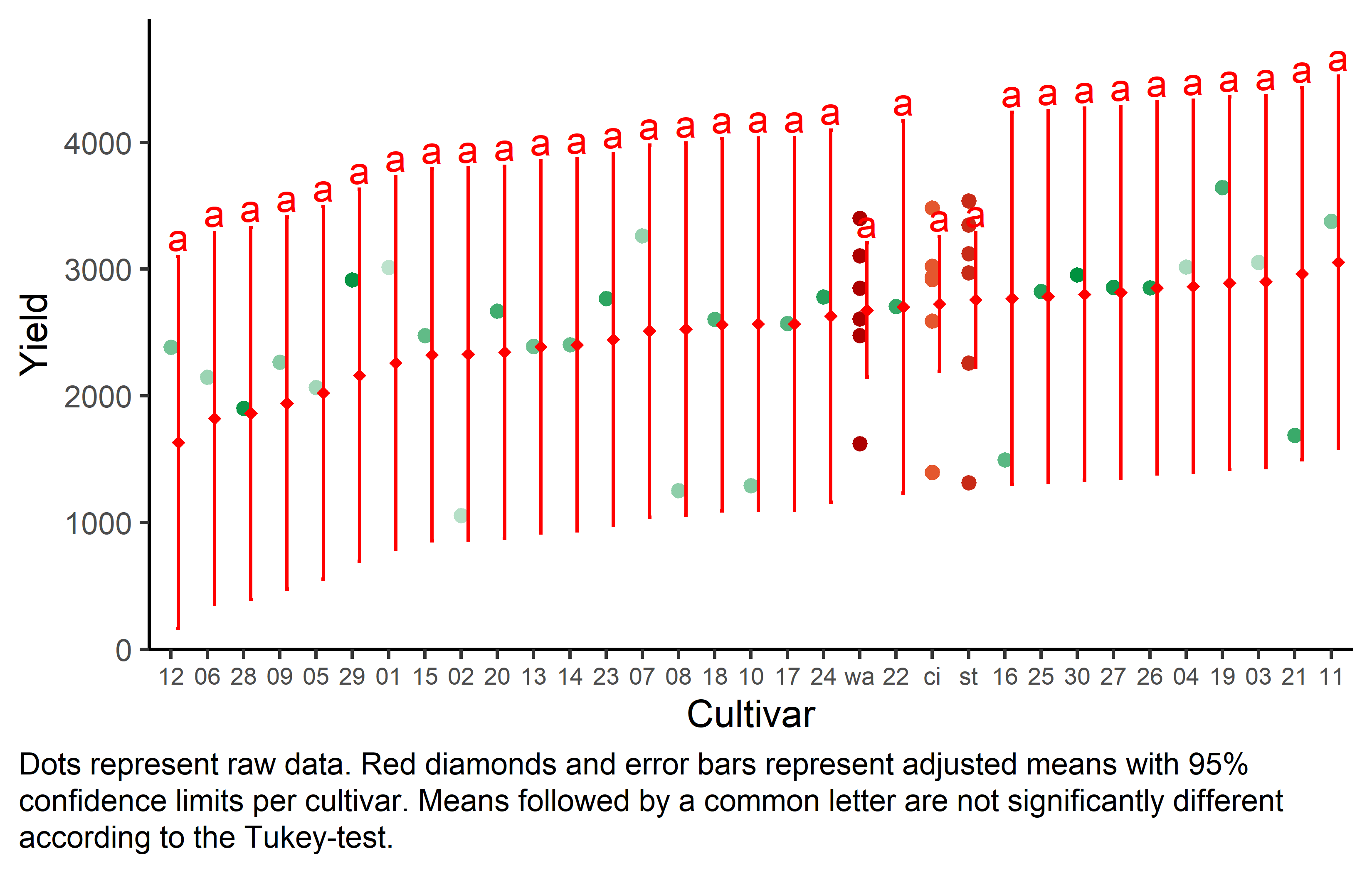
Bonus
Here are some other things you would maybe want to look at for the analysis of this dataset.
Variance components
To extract variance components from our models, we unfortunately need different functions per model since only of of them is a mixed model and we used different functions to fit them.
# Residual Variance
summary(mod_fb)$sigma^2
[1] 91102.66# Both Variance Components
as_tibble(VarCorr(mod_rb))# A tibble: 2 × 5
grp var1 var2 vcov sdcor
<chr> <chr> <chr> <dbl> <dbl>
1 block (Intercept) <NA> 434198. 659.
2 Residual <NA> <NA> 91103. 302.References
Citation
@online{schmidt2023,
  author = {Paul Schmidt},
  title = {One-Way Augmented Design},
  date = {2023-11-18},
  url = {https://schmidtpaul.github.io/dsfair_quarto//ch/exan/simple/augm_petersen1994.html},
  langid = {en},
  abstract = {One-way ANOVA \& pairwise comparison post hoc tests in a
    non-resolvable augmented design.}
}