⚠ Hey, nice that you're here! BUT...
This site is no longer maintained and may contain outdated information.
I'm keeping it online because I once promised to never take it down –
but I've since built a much better, up-to-date resource. I'd really
appreciate if you checked it out and found the corresponding chapter there: ➔ biomathcontent.netlify.app
⚠ Hi, schön, dass du hier bist, ABER...
Diese Seite wird nicht mehr gepflegt und enthält möglicherweise
veraltete Informationen. Ich habe versprochen sie online zu lassen,
also bleibt sie stehen – aber alle Inhalte wurden überarbeitet,
verbessert und auf einer neuen Seite zusammengeführt.
Schau bitte stattdessen dort vorbei: ➔ biomathcontent.netlify.app
A personal collection of useful R packages and more.
This chapter is a collection of things I wish I had known earlier in my years using R and that I hope can be of use to you. Sections are named after R packages or whatever applies and sorted alphabetically.
{broom}
In R, results from statistical tests, models etc. are often formatted in a way that may not be optimal for further processing steps. Luckily, {broom} will format the results of the most common functions into tidy data structures.
# Correlation Analysis for built-in example data "mtcars"mycor<-cor.test(mtcars$mpg, mtcars$disp)mycor
    Pearson's product-moment correlation

data:  mtcars$mpg and mtcars$disp
t = -8.7472, df = 30, p-value = 9.38e-10
alternative hypothesis: true correlation is not equal to 0
95 percent confidence interval:
 -0.9233594 -0.7081376
sample estimates:
       cor
-0.8475514
Sometimes, different packages have different functions with identical names. A famous example is the function filter(), which exists in {stats} and {dplyr}. If both of these packages are loaded, it is not clear which of the two functions should be used. This is called a function conflict and it is especially tricky here since {stats} is always loaded. By default, R will simply pick the package that was loaded later - which is obviously not optimal.
One way of dealing with function conflicts is by using the packagename::functionname() method, because when writing dplyr::filter() instead of filter() it is no longer ambiguous which function you are referring to.
Another way of dealing with function conflicts more explicitly is by loading the {conflicted} package. Once it is loaded, function conflicts will lead to an Error that forces you to deal with the issue:
Error:
! [conflicted] filter found in 2 packages.
Either pick the one you want with `::`:
• dplyr::filter
• stats::filter
Or declare a preference with `conflicts_prefer()`:
• `conflicts_prefer(dplyr::filter)`
• `conflicts_prefer(stats::filter)`
As you can see, it first suggests using the packagename::functionname() method mentioned above, but also points to the conflict_prefer() function. By running this function once in the beginning of the script, R will always use the function from the package that you declared the “winner”:
{desplot} makes it easy to plot experimental designs of field trials in agriculture. However, you do need two columns that provide the x and y coordinates of the individual plots on your field.
TO DO
{dlookr}
When providing descriptive statistics tables, one may find the number of relevant measures become annoyingly large so that even with the {tidyverse}, several lines of code are necessary. Here are just five measures, and they are not even including the na.rm = TRUE argument, which is necessary for data with missing values.
# A tibble: 3 × 6
  group  mean stddev median   min   max
  <fct> <dbl>  <dbl>  <dbl> <dbl> <dbl>
1 ctrl   5.03  0.583   5.15  4.17  6.11
2 trt1   4.66  0.794   4.55  3.59  6.03
3 trt2   5.53  0.443   5.44  4.92  6.31
Obviously, there are multiple packages who try to address just that. The one I’ve been using for some time now is {dlookr} with its describe() function. It actually provides more measures than I usually need1, but it has everything I want and I disregard the rest (via select()).
It is intentional that I did not actually load the {dlookr} package, but instead used its describe() function via the packagename::functionname() method. This is because of a minor bug in the {dlookr} package described here, which is only relevant if you are using the package with knitr/Rmarkdown/quarto. I am using quarto to generate this website and thus I avoid loading the package. This is fine for me, since I usually only need this one function one time during an analysis. It is also fine for you, since the code works the same way in a standard R script.
{ggtext}
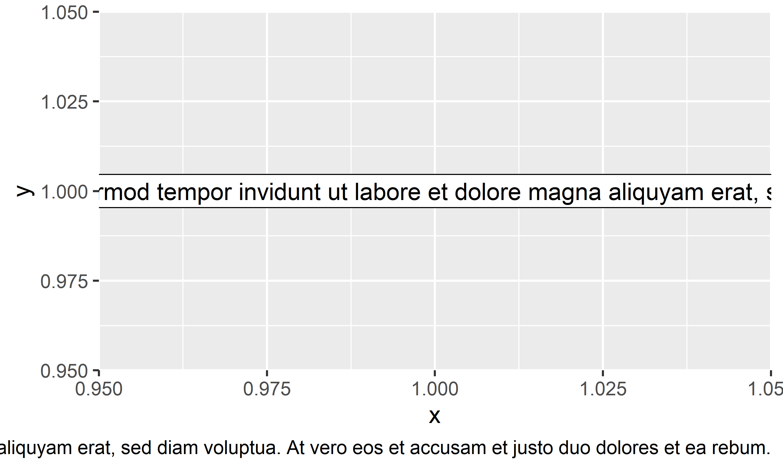
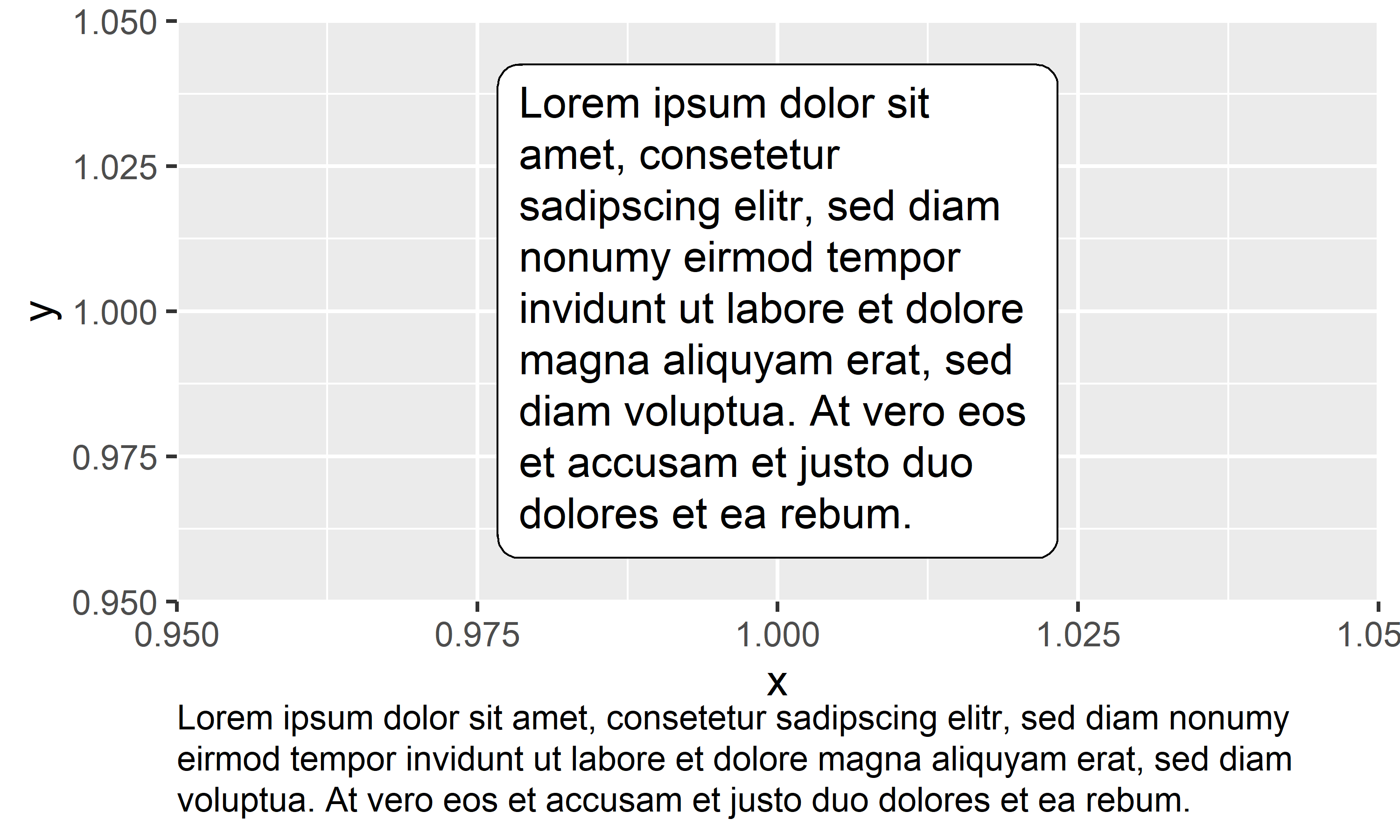
Adding long text to plots created via {ggplot2} is problematic, since you have to insert line breaks yourself. However, {ggext}’s geom_textbox() for data labels and element_textbox_simple() for title, caption etc. will automatically add line breaks:
longtext<-"Lorem ipsum dolor sit amet, consetetur sadipscing elitr, sed diam nonumy eirmod tempor invidunt ut labore et dolore magna aliquyam erat, sed diam voluptua. At vero eos et accusam et justo duo dolores et ea rebum."
You now know how to install and load R packages the standard way. However, over the years I switched to using the function p_load() from the {pacman} package instead of library() and install.packages(). The reason is simple: Usually R-scripts start with multiple lines of library() statements that load the necessary packages. However, when this code is run on a different computer, the user may not have all these packages installed and will therefore get an error message. This can be avoided by using the p_load(), because it
loads all packages that are installed and
installs and loads all packages that are not installed.
Obviously, {pacman} itself must first be installed (the standard way). Moreover, you may now think that in order to use p_load() we do need a single library(pacman) first. However, we can avoid this by writing pacman::p_load() instead. Simply put, writing package_name::function_name()makes sure that this explicit function from this explicit package is being used. Additionally, R actually lets you use this function without loading the corresponding package. Thus, we now arrived at the way I handle packages at the beginning of all my R-scripts:
Not built-in, for some reason, is the opposite of that function - checking whether something is not present. Yet, we can quickly built our own function that does exactly that:
Keep in mind that p00 is the 0th percentile and thus the minimum. Analogously, p50 is the median and p100 the maximum.↩︎
Citation
BibTeX citation:
@online{schmidt2023,
  author = {Paul Schmidt},
  title = {Useful Things},
  date = {2023-11-07},
  url = {https://schmidtpaul.github.io/dsfair_quarto//ch/misc/usefulthings.html},
  langid = {en},
  abstract = {A personal collection of useful R packages and more.}
}
---title: "Useful things"abstract: "A personal collection of useful R packages and more."---```{r}#| include: falsesource(here::here("src/helpersrc.R"))```This chapter is a collection of things I wish I had known earlier in my years using R and that I hope can be of use to you. Sections are named after R packages or whatever applies and sorted alphabetically.# `{broom}`In R, results from statistical tests, models etc. are often formatted in a way that may not be optimal for further processing steps. Luckily, [{broom}](https://broom.tidymodels.org/) will format the results of [the most common functions](https://broom.tidymodels.org/articles/available-methods.html) into [tidy data structures](https://www.jstatsoft.org/article/view/v059i10).```{r}# Correlation Analysis for built-in example data "mtcars"mycor <-cor.test(mtcars$mpg, mtcars$disp)mycorlibrary(broom)tidy(mycor)```# `{conflicted}`Sometimes, different packages have different functions with identical names. A famous example is the function `filter()`, which exists in [{stats}](https://www.rdocumentation.org/packages/stats/versions/3.6.2/topics/filter) and [{dplyr}](https://dplyr.tidyverse.org/reference/filter.html). If both of these packages are loaded, it is not clear which of the two functions should be used. This is called a function conflict and it is especially tricky here since {stats} is always loaded. By default, R will simply pick the package that was loaded later - which is obviously not optimal.One way of dealing with function conflicts is by using the [packagename::functionname()](https://stackoverflow.com/questions/35240971/what-are-the-double-colons-in-r) method, because when writing `dplyr::filter()` instead of `filter()` it is no longer ambiguous which function you are referring to.Another way of dealing with function conflicts more explicitly is by loading the {conflicted} package. Once it is loaded, function conflicts will lead to an `Error` that forces you to deal with the issue:```{r}#| error: truelibrary(conflicted)library(dplyr)PlantGrowth %>%filter(weight >6)```As you can see, it first suggests using the [packagename::functionname()](https://stackoverflow.com/questions/35240971/what-are-the-double-colons-in-r) method mentioned above, but also points to the `conflict_prefer()` function. By running this function once in the beginning of the script, R will always use the function from the package that you declared the "winner":```{r}library(conflicted)library(dplyr)conflicts_prefer(dplyr::filter)PlantGrowth %>%filter(weight >6)```# `{desplot}`[{desplot}](https://kwstat.github.io/desplot/) makes it easy to plot experimental designs of field trials in agriculture. However, you do need two columns that provide the x and y coordinates of the individual plots on your field.TO DO# `{dlookr}`When providing descriptive statistics tables, one may find the number of relevant measures become annoyingly large so that even with the {tidyverse}, several lines of code are necessary. Here are just five measures, and they are not even including the [`na.rm = TRUE`](https://www.statology.org/na-rm/) argument, which is necessary for data with missing values.```{r}library(tidyverse)PlantGrowth %>%group_by(group) %>%summarise(mean =mean(weight),stddev =sd(weight),median =median(weight),min =min(weight),max =max(weight) )```Obviously, there are multiple packages who try to address just that. The one I've been using for some time now is [{dlookr}](https://choonghyunryu.github.io/dlookr/) with its `describe()` function. It actually provides more measures than I usually need[^1], but it has everything I want and I disregard the rest (via `select()`).[^1]: Keep in mind that `p00` is the 0th percentile and thus the minimum. Analogously, `p50` is the median and `p100` the maximum.```{r}PlantGrowth %>%group_by(group) %>% dlookr::describe(weight)```::: callout-noteIt is intentional that I did not actually load the {dlookr} package, but instead used its `describe()` function via the [packagename::functionname()](https://stackoverflow.com/questions/35240971/what-are-the-double-colons-in-r) method. This is because of a minor bug in the {dlookr} package described [here](https://github.com/choonghyunryu/dlookr/issues/79), which is only relevant if you are using the package with knitr/Rmarkdown/quarto. I am using quarto to generate this website and thus I avoid loading the package. This is fine for me, since I usually only need this one function one time during an analysis. It is also fine for you, since the code works the same way in a standard R script.:::# `{ggtext}`Adding long text to plots created via {ggplot2} is problematic, since you have to insert line breaks yourself. However, [{ggext}](https://wilkelab.org/ggtext/)'s `geom_textbox()` for data labels and `element_textbox_simple()` for title, caption etc. will automatically add line breaks:```{r}longtext <-"Lorem ipsum dolor sit amet, consetetur sadipscing elitr, sed diam nonumy eirmod tempor invidunt ut labore et dolore magna aliquyam erat, sed diam voluptua. At vero eos et accusam et justo duo dolores et ea rebum."```::: columns::: {.column width="49%"}```{r}#| fig-width: 5#| fig-height: 3library(ggplot2)ggplot() +aes(y =1, x =1, label = longtext) +geom_label() +labs(caption = longtext)```:::::: {.column width="2%"}:::::: {.column width="49%"}```{r}#| fig-width: 5#| fig-height: 3library(ggtext)ggplot() +theme(plot.caption =element_textbox_simple()) +aes(y =1, x =1, label = longtext) +geom_textbox() +labs(caption = longtext)```::::::# `{here}`TO DO# `{insight}`[TO DO](https://easystats.github.io/insight/reference/format_p.html)# `{janitor}`TO DO# Keyboard shortcutsHere are shortcuts I actually use regularly in RStudio:| Shortcut | Description ||-----------------------|-----------------------------------------------|| CTRL+ENTER | Run selected lines of code || CTRL+C | Convert all selected lines to comment || CTRL+SHIFT+M | Insert `%>%` || CTRL+SHIFT+R | Insert code section header || CTRL+LEFT/RIGHT | Jump to Word || CTRL+SHIFT+LEFT/RIGHT | Select Word || ALT+LEFT/RIGHT | Jump to Line Start/End || ALT+SHIFT+LEFT/RIGHT | Select to Line Start/End || CTRL+A | Highlight everything (to run the entire code) || CTRL+Z | Undo |Keyboard shortcuts can be customized in RStudio as described [here](https://support.rstudio.com/hc/en-us/articles/206382178-Customizing-Keyboard-Shortcuts-in-the-RStudio-IDE).# `{modelbased}`[TO DO](https://easystats.github.io/modelbased/articles/estimate_response.html)# `{openxlsx}`TO DO# `{pacman}`[<img src="https://github.com/trinker/pacman/blob/master/inst/pacman_logo/r_pacman.png?raw=true" width="100"/>](https://tidyverse.tidyverse.org/)You now know how to install and load R packages the standard way. However, over the years I switched to using the function `p_load()` from the {pacman} package instead of `library()` and `install.packages()`. The reason is simple: Usually R-scripts start with multiple lines of `library()` statements that load the necessary packages. However, when this code is run on a different computer, the user may not have all these packages installed and will therefore get an error message. This can be avoided by using the `p_load()`, because it- loads all packages that are installed and- installs and loads all packages that are not installed.Obviously, {pacman} itself must first be installed (the standard way). Moreover, you may now think that in order to use `p_load()` we do need a single `library(pacman)` first. However, we can avoid this by writing `pacman::p_load()` instead. Simply put, writing `package_name::function_name()`[makes sure](https://stat.ethz.ch/R-manual/R-devel/library/base/html/ns-dblcolon.html) that this explicit function from this explicit package is being used. Additionally, R actually lets you use this function without loading the corresponding package. Thus, we now arrived at the way I handle packages at the beginning of all my R-scripts:```{r}#| eval: falsepacman::p_load( package_name_1, package_name_2, package_name_3)```# `{patchwork}`TO DO# `{performance}`TO DO# `{readxl}`TO DO# `{reprex}`TO DO# `{scales}`TO DO# `%in%` and `%not_in%`R has the built-in function `%in%` which checks whether something is present in a vector.```{r}treatments <-c("Ctrl", "A", "B")```Not only can we checke which treatments are present in our `treatment` vector (left), but we can also easily keep only those that are (right).::: columns::: {.column width="49%"}```{r}c("A", "D") %in% treatments ```:::::: {.column width="2%"}:::::: {.column width="49%"}```{r}c("A", "D") %>% .[. %in% treatments]```::::::Not built-in, for some reason, is the opposite of that function - checking whether something is **not** present. Yet, we can quickly built our own function that does exactly that:```{r}`%not_in%`<-Negate(`%in%`)```::: columns::: {.column width="49%"}```{r}c("A", "D") %not_in% treatments ```:::::: {.column width="2%"}:::::: {.column width="49%"}```{r}c("A", "D") %>% .[. %not_in% treatments]```::::::# `system('open "file.png"')`[TO DO](https://gist.github.com/SchmidtPaul/5cd96b53449f5f50cbda725d4cdacf9b)