Designing experiments
In this summary {agricolae} is used to generate a few common experimental designs based on a given number of treatment factor levels and a number of desired replicates (see “Example Setup” below). Additionally, each experimental design that was generated is also plotted using {desplot} so that different designs can be compared easily.
# packages
pacman::p_load(tidyverse, # data handling
               agricolae, # experimental design
               desplot)   # plots
Example Setup
# 2 pesiticides
TrtPest   <- paste0("P", 1:2)    # P1 & P2
n_TrtPest <- n_distinct(TrtPest) # 2

# 4 soil treatments
TrtSoil   <- paste0("S", 1:4)    # S1 - S4
n_TrtSoil <- n_distinct(TrtSoil) # 4

# 6 fertilizer
TrtFert   <- paste0("N", 1:6)    # N1 - N6
n_TrtFert <- n_distinct(TrtFert) # 6

# 15 genotpyes
TrtGen    <- paste0("G", 1:15)   # G1 - G15
n_TrtGen  <- n_distinct(TrtGen)  # 15

# 2 check varieties
Checks    <- c("Std_A", "Std_B")

# number of replicates
n_Reps    <- 3
One treatment factor
CRD
completely randomized design
crd_out <- design.crd(trt = TrtSoil,
                      r = n_Reps,
                      seed = 42)

# Add Row and Col
crd_out$bookRowCol <- crd_out$book %>%
  bind_cols(expand.grid(Row = 1:n_Reps,
                        Col = 1:n_TrtSoil))

# Plot field layout
desplot(TrtSoil ~ Row + Col, flip = TRUE,
        text = TrtSoil, cex = 1, shorten = "no",
        data = crd_out$bookRowCol,
        main = "completely randomized design",
        show.key = F)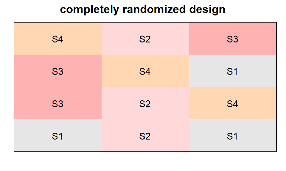
RCBD
randomized complete block design
rcbd_out <- design.rcbd(trt = TrtSoil,
                        r = n_Reps,
                        seed = 42)

# Add Row and Col
rcbd_out$bookRowCol <- rcbd_out$book %>%
  mutate(Row = block %>% as.integer) %>%
  group_by(Row) %>%
  mutate(Col = 1:n()) %>%
  ungroup()

# Plot field layout
desplot(TrtSoil ~ Row + Col, flip = TRUE,
        text = TrtSoil, cex = 1, shorten = "no",
        out1 = block,
        data = rcbd_out$bookRowCol,
        main = "randomized complete block design",
        show.key = T, key.cex = 0.5)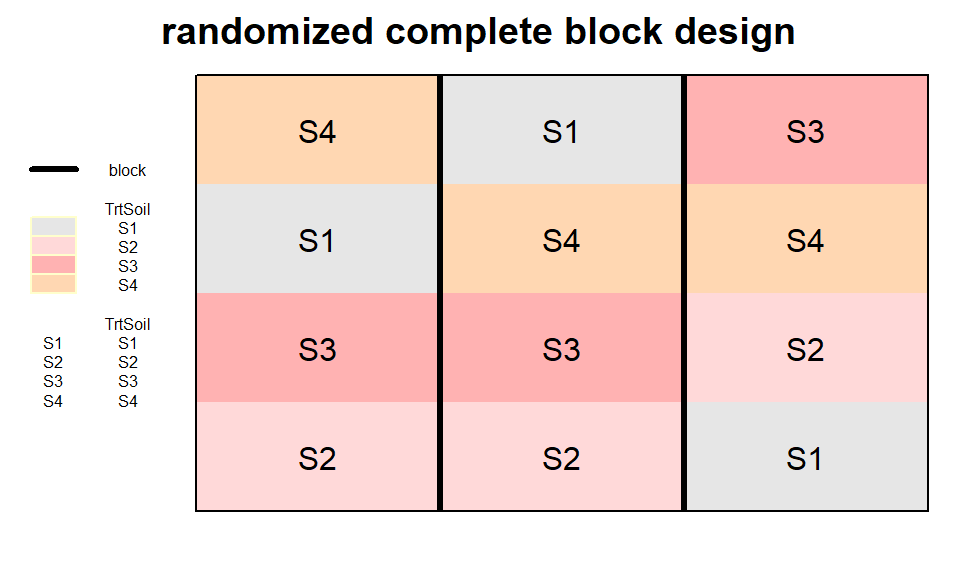
latin square design
latsquare_out <- design.lsd(trt = TrtSoil,
                            seed = 42)

# Add Row and Col
latsquare_out$bookRowCol <- latsquare_out$book %>%
  mutate(Row = row %>% as.integer,
         Col = col %>% as.integer)

# Plot field layout
desplot(TrtSoil ~ Row + Col, flip = TRUE,
        out1 = Row, out1.gpar=list(col="black", lwd=3),
        out2 = Col, out2.gpar=list(col="black", lwd=3),
        text = TrtSoil, cex = 1, shorten = "no",
        data = latsquare_out$bookRowCol,
        main = "latin square design",
        show.key = T, key.cex = 0.5)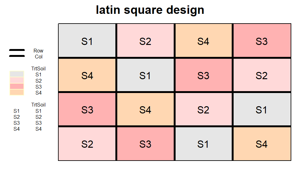
alpha design
alpha_out <- design.alpha(trt = TrtGen,
                          k = 3,
                          r = n_Reps,
                          seed = 42)

# Add Row and Col
alpha_out$bookRowCol <- alpha_out$book %>%
  mutate(replication = paste0("Rep", replication),
         Row = block %>% as.integer,
         Col = cols  %>% as.integer)

# Plot field layout
desplot(TrtGen ~ Row + Col | replication, flip = TRUE,
        out1 = replication,
        out2 = block, out2.gpar = list(col = "black", lty = 3),
        text = TrtGen, cex = 1, shorten = "no",
        data = alpha_out$bookRowCol,
        main = "alpha design",
        show.key = F)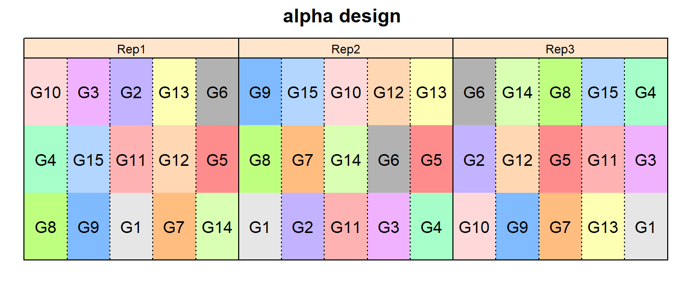
augmented design
augmented_out <- design.dau(trt1 = Checks,
                            trt2 = TrtGen,
                            r = n_Reps,
                            seed = 42)

# Add Row and Col
augmented_out$bookRowCol <- augmented_out$book %>%
  mutate(Col = block %>% as.integer,
         Row = plots %>% str_sub(3,3) %>% as.integer)

# Plot field layout
desplot(trt ~ Row + Col, flip = TRUE,
        out1 = block, out1.gpar = list(col = "black", lwd = 2, lty = 3),
        text = trt, cex = 1, shorten = "no",
        data = augmented_out$bookRowCol ,
        main = "augmented design",
        show.key = F)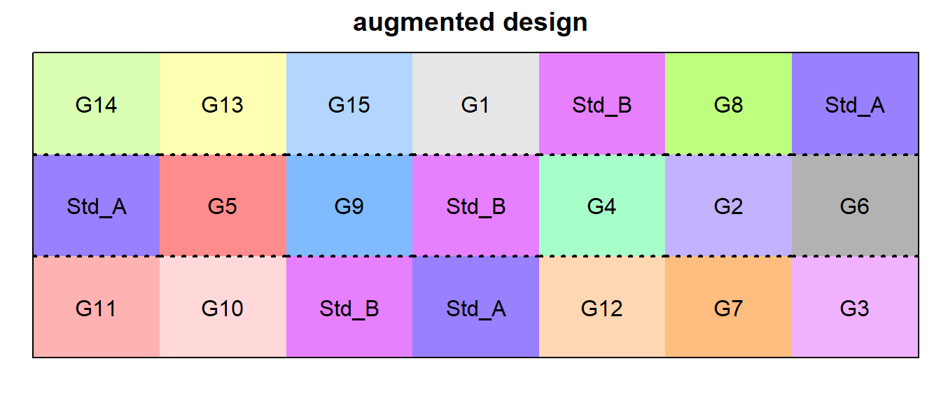
Two treatment factors
Factorial: You have at least two treatment factors, and all levels of each factor are used in combination with all other factor levels. These factors are said to be cross-classified, as opposed to nested. Additionally, each of the resulting treatment combinations is applied to the same type of experimental unit.
RCBD (factorial)
fac2rcbd_out <- design.ab(trt = c(n_TrtFert, n_TrtSoil),
                          design = "rcbd",
                          r = n_Reps,
                          seed = 42)

# Add Row and Col
fac2rcbd_out$bookRowCol <- fac2rcbd_out$book %>%
  bind_cols(expand.grid(Row = 1:n_TrtFert,
                        Col = 1:(n_TrtSoil*n_Reps))) %>%
  mutate(TrtFert = paste0("N", A),
         TrtSoil = paste0("S", B))

# Plot field layout
desplot(block ~ Col + Row | block, flip = TRUE,
        out1 = Row, out1.gpar = list(col = "grey", lty = 1),
        out2 = Col, out2.gpar = list(col = "grey", lty = 1),
        text = TrtFert, cex = 1, shorten = "no", col=TrtSoil,
        data = fac2rcbd_out$bookRowCol,
        main = "RCBD",
        show.key = T, key.cex = 0.5)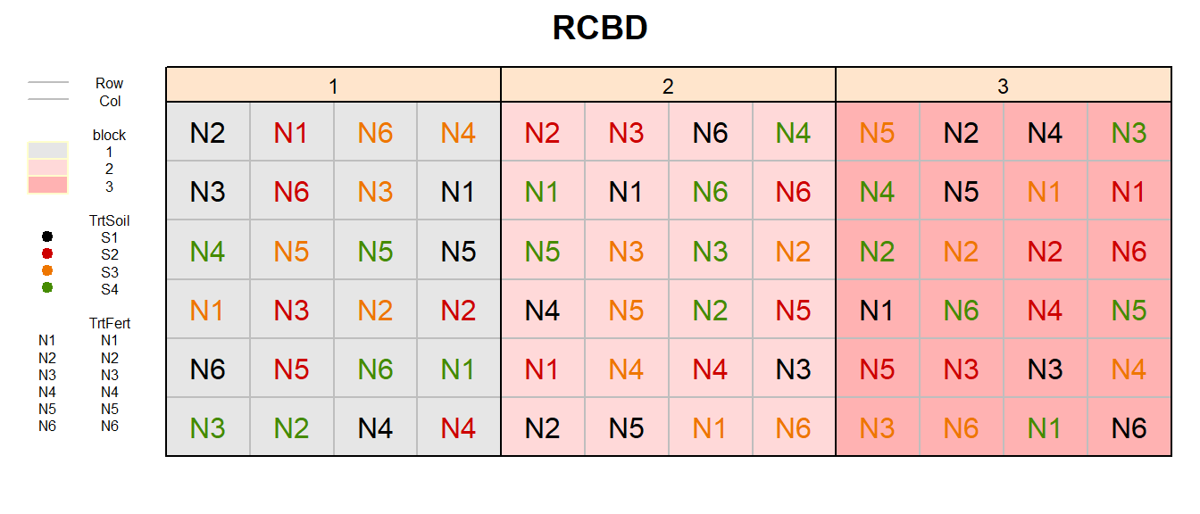
split plot design
splitplot_out <- design.split(trt1 = TrtSoil,
                              trt2 = TrtFert,
                              r = n_Reps,
                              seed = 42)

# Add Row and Col
splitplot_out$bookRowCol <- splitplot_out$book %>%
  mutate(block = paste0("Block", block),
         Col   = plots %>% str_sub(2,3) %>% as.integer,
         Row   = splots %>% as.integer)

# Plot field layout
desplot(block ~ Col + Row | block, flip = TRUE,
        out1 = Row, out1.gpar = list(col = "grey", lty = 1),
        out2 = Col, out2.gpar = list(col = "grey", lty = 1),
        text = TrtFert, cex = 1, shorten = "no", col=TrtSoil,
        data = splitplot_out$bookRowCol ,
        main = "split plot design",
        show.key = T, key.cex = 0.5)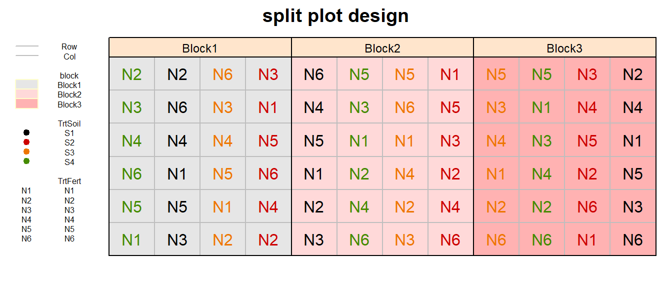
Three treatment factors
RCBD (factorial)
fac3rcbd_out <- design.ab(trt = c(n_TrtPest, n_TrtFert, n_TrtSoil),
                          design = "rcbd",
                          r = n_Reps,
                          seed = 42)

# Add Row and Col
fac3rcbd_out$bookRowCol <- fac3rcbd_out$book %>%
  bind_cols(expand.grid(Row = 1:(n_TrtFert*n_TrtPest),
                        Col = 1:(n_TrtSoil*n_Reps))) %>%
  mutate(block   = paste0("Block", block),
         TrtPest = paste0("P", A),
         TrtFert = paste0("N", B),
         TrtSoil = paste0("S", C))

# Plot field layout
desplot(TrtPest ~ Col + Row | block, flip = TRUE,
        out1 = Row, out1.gpar = list(col = "grey", lty = 1),
        out2 = Col, out2.gpar = list(col = "grey", lty = 1),
        text = TrtFert, cex = 1, shorten = "no", col = TrtSoil,
        data = fac3rcbd_out$bookRowCol,
        main = "RCBD",
        show.key = T, key.cex = 0.5)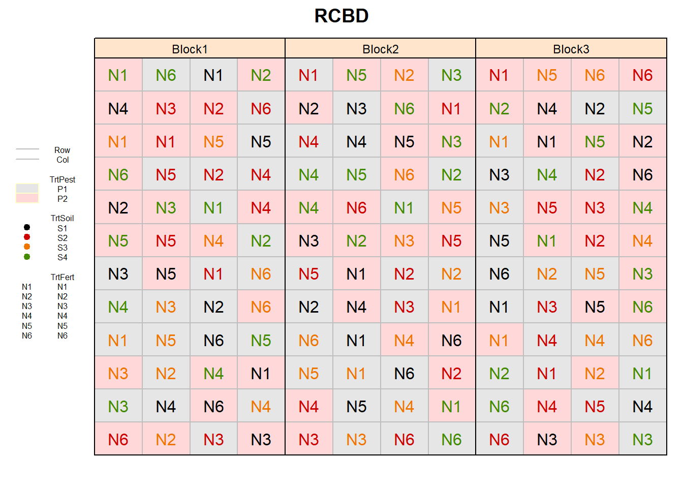
Please feel free to contact me about any of this!
schmidtpaul1989@outlook.com