Repeated Measures RCBD
# packages

# the package "mixedup" is not on CRAN, so that you must install
# it once with the following code:
withr::with_envvar(c(R_REMOTES_NO_ERRORS_FROM_WARNINGS = "true"),
  remotes::install_github('m-clark/mixedup')
)

pacman::p_load(agriTutorial, tidyverse,  # data import and handling
               conflicted, # handle conflicting functions
               nlme, glmmTMB, # linear mixed modelling
               mixedup, AICcmodavg, car, # linear mixed model processing
               emmeans, multcomp, multcompView, # mean comparisons
               ggplot2, gganimate, gifski)  # (animated) plots

conflict_prefer("select", "dplyr") # set select() from dplyr as default
conflict_prefer("filter", "dplyr") # set filter() from dplyr as default
Data
The example in this chapter is taken from Example 4 in Piepho & Edmondson (2018)
(see also the Agritutorial vigniette). It considers data from a
sorghum trial laid out as a randomized complete block
design (5 blocks) with variety (4 sorghum varities) being
the only treatment factor. Thus, we have a total of 20
plots. It is important to note that our response variable
(y), the leaf area index, was assessed in five
consecutive weeks on each plot starting 2 weeks after
emergence. Therefore, the dataset contains a total of 100 values and
what we have here is longitudinal data, a.k.a. repeated
measurements over time, a.k.a. a time series analysis.
As Piepho & Edmondson (2018) put it: “the week factor is not a treatment factor that can be randomized. Instead, repeated measurements are taken on each plot on five consecutive occasions. Successive measurements on the same plot are likely to be serially correlated, and this means that for a reliable and efficient analysis of repeated-measures data we need to take proper account of the serial correlations between the repeated measures (Piepho, Büchse & Richter, 2004; Pinheiro & Bates, 2000).”
Please note that this example is also considered on the MMFAIR website but with more focus on how to use the different mixed model packages to fit the models.
Import & Formatting
Note that I here decided to give more intuitive names and labels, but
this is optional. We also create a column unit with one
factor level per observation, which will be needed later when using
glmmTMB().
# data - reformatting agriTutorial::sorghum
dat <- agriTutorial::sorghum %>% # data from agriTutorial package
  rename(block = Replicate,
         weekF = factweek,  # week as factor
         weekN = varweek,   # week as numeric/integer
         plot  = factplot) %>%
  mutate(variety = paste0("var", variety),    # variety id
         block   = paste0("block", block),    # block id
         weekF   = paste0("week", weekF),     # week id
         plot    = paste0("plot", plot),      # plot id
         unit    = paste0("obs", 1:n() )) %>% # obsevation id
  mutate_at(vars(variety:plot, unit), as.factor) %>%
  as_tibble()

dat
## # A tibble: 100 × 8
## y variety block weekF plot weekN varblock unit
## <dbl> <fct> <fct> <fct> <fct> <int> <int> <fct>
## 1 5 var1 block1 week1 plot1 1 1 obs1
## 2 4.84 var1 block1 week2 plot1 2 1 obs2
## 3 4.02 var1 block1 week3 plot1 3 1 obs3
## 4 3.75 var1 block1 week4 plot1 4 1 obs4
## 5 3.13 var1 block1 week5 plot1 5 1 obs5
## 6 4.42 var1 block2 week1 plot2 1 2 obs6
## 7 4.3 var1 block2 week2 plot2 2 2 obs7
## 8 3.67 var1 block2 week3 plot2 3 2 obs8
## 9 3.23 var1 block2 week4 plot2 4 2 obs9
## 10 2.83 var1 block2 week5 plot2 5 2 obs10
## # … with 90 more rowsExploring
In order to obtain a field layout of the trial, we would like use the
desplot() function. Notice that for this we need two data
columns that identify the row and col of each
plot in the trial. These are unfortunately not given here, so that we
cannot create the actual field layout plot.
descriptive tables
We could also have a look at the arithmetic means and standard
deviations for yield per variety.
dat %>%
  group_by(variety) %>%
  summarize(mean    = mean(y, na.rm=TRUE),
            std.dev = sd(y, na.rm=TRUE)) %>%
  arrange(desc(mean)) %>% # sort
  print(n=Inf) # print full table
## # A tibble: 4 × 3
## variety mean std.dev
## <fct> <dbl> <dbl>
## 1 var3 4.63 0.757
## 2 var4 4.61 0.802
## 3 var2 4.59 0.763
## 4 var1 3.50 0.760Furthermore, we could look at the arithmetic means for each week as follows:
dat %>%
  group_by(weekF, variety) %>%
  summarize(mean = mean(y, na.rm=TRUE)) %>%
  pivot_wider(names_from = weekF, values_from = mean)
## # A tibble: 4 × 6
## variety week1 week2 week3 week4 week5
## <fct> <dbl> <dbl> <dbl> <dbl> <dbl>
## 1 var1 4.24 4.05 3.41 3.09 2.7
## 2 var2 5.15 4.98 4.59 4.22 4.01
## 3 var3 4.89 5.07 4.71 4.48 4.02
## 4 var4 5.15 4.94 4.71 4.39 3.83descriptive plot
We can also create a plot to get a better feeling for the data. Note that here we could even decide to extend the ggplot to become an animated gif as follows:
var_colors <- c("#8cb369", "#f4a259", "#5b8e7d", "#bc4b51")
names(var_colors) <- dat$variety %>% levels()

gganimate_plot <- ggplot(
  data = dat, aes(y = y, x = weekF,
                  group = variety,
                  color = variety)) +
  geom_boxplot(outlier.shape = NA) +
  geom_point(alpha = 0.5, size = 3) +
  scale_y_continuous(
    name = "Leaf area index",
    limits = c(0, 6.5),
    expand = c(0, 0),
    breaks = c(0:6)
  ) +
  scale_color_manual(values = var_colors) +
  theme_bw() +
  theme(legend.position = "bottom",
        axis.title.x = element_blank()) +
  transition_time(weekN) +
  shadow_mark(exclude_layer = 2)

animate(gganimate_plot, renderer = gifski_renderer()) # render gif
Model building
Our goal is therefore to build a suitable model taking serial correlation into account. In order to do this, we will initially consider the model for a single time point. Then, we extend this model to account for multiple weeks by allowing for week-speficic effects. Finally, we further allow for serially correlated error terms.
Single week
When looking at data from a single time point (e.g. the
first week), we merely have 20 observations from a randomized complete
block design with a single treatment factor. It can therefore be
analyzed with a simple one-way ANOVA (fixed variety effect)
for randomized complete block designs (fixed block
effect):
dat.wk1 <- dat %>% filter(weekF == "week1") # subset data from first week only

mod.wk1 <- lm(formula = y ~ variety + block,
              data = dat.wk1)
We could now go on and look at the ANOVA via
anova(mod.wk1) and it would indeed not be wrong to
simply repeat this for each week. Yet, one may not be satisfied with
obtaining multiple ANOVA results - namely one per week. This is
especially likeliy in case the results contradict each other, because
e.g. the variety effects are found to be significant in only
two out of five weeks. Therefore, one may want to analyze the entire
dataset i.e. the multiple weeks jointly.
Multiple weeks (MW)
Going from the single-week-analysis to jointly analyzing the entire
dataset is more than just changing the data = statement in
the model. This is because “it is realistic to assume that the
treatment effects evolve over time and thus are week-specific.
Importantly, we must also allow for the block effects to change over
time in an individual manner. For example, there could be fertility or
soil type differences between blocks and these could have a smooth
progressive or cumulative time-based effect on differences between the
blocks dependent on factors such as temperature or rainfall” (Piepho & Edmondson, 2018). We implement this by
taking the model in mod.wk1 and multipyling each effect
with week. Note that this is also true for the general
interecept (µ) in mod.wk1, meaning that we would like to
include one intercept per week, which can be achieved by simply adding
week as a main effect as well. This leaves us with fixed
main effects for week, variety, and
block, as well as the week-specific effects of the latter
two week:variety and week:block.
Finally, note that we are not doing anything about the model’s error term at this point. More specifically this means that its variance structure is still the default iid (independent and identically distributed) - see the summary on correlation/variance strucutres at the MMFAIR website.
I decide to use the
glmmTMBpackage to fit the linear models here, because I feel that their syntax is more intuitive. Note that one may also use thenlmepackage to do this, just as (Piepho & Edmondson, 2018) did and you can find a direct comparison of the R syntax with additional information in the MMFAIR chapter.
MW - indepentent errors
glmmTMB
With the glmmTMB() function, it is possible to
- fix the error variance to 0 via adding the
dispformula = ~ 0argument and then - mimic the error (variance) as a random effect (variance) via the
unitcolumn with different entries for each data point.
While this may not be necessary for this model with the default homoscedastic, independent error variance structure, using it here will allow for an intuitve comparison to the following model with more sophisticated variance structures.
mod.iid <- glmmTMB(formula = y ~ weekF * (variety + block)
                        + (1 | unit),      # add random unit term to mimic error variance
                        dispformula = ~ 0, # fix original error variance to 0
                        REML = TRUE,       # needs to be stated since default = ML
                        data = dat)

# Extract variance component estimates
# alternative: mod.iid %>% broom.mixed::tidy(effects = "ran_pars", scales = "vcov")
mod.iid %>% mixedup::extract_vc(ci_scale = "var")
## # A tibble: 2 × 7
## group effect variance sd var_2.5 var_97.5 var_prop
## <chr> <chr> <dbl> <dbl> <dbl> <dbl> <dbl>
## 1 unit Intercept 0.023 0.152 0.016 0.033 1
## 2 Residual <NA> 0 0 NA NA 0As expected, we find the residual variance to be 0 and instead we
have the mimiced homoscedastic, independent error variance for the
random (1 | unit) effect estimated as 0.023.
nlme
Since the models in this chapter do not contain any random effects,
we make use of gls() instead of lme().
Furthermore, we specifically write out the
correlation = NULL argument to get a homoscedastic,
independent error variance structure. While this may not be necessary
because it is the default, using it here will allow for an intuitve
comparison to the following models with more sophisticated variance
structures.
mod.iid.nlme <- gls(model = y ~ weekF * (block + variety),
                    correlation = NULL, # default, i.e. homoscedastic, independent errors
                    data = dat)

# Extract variance component estimates
tibble(varstruct = "iid") %>%
  mutate(sigma    = mod.iid.nlme$sigma) %>%
  mutate(Variance = sigma^2)
## # A tibble: 1 × 3
## varstruct sigma Variance
## <chr> <dbl> <dbl>
## 1 iid 0.152 0.0232It can be seen that the residual homoscedastic, independent error variance was estimated as 0.023.
MW - autocorrelated errors
Note that at this point of the analysis, the model above with an
independent, homogeneous error term above is neither the right, nor the
wrong choice. It must be clear that “measurements on the same plot
are likely to be serially correlated”. Thus, it
should be investigated whether any covariance structure for the error
term (instead of the default independence between errors) is more
appropriate to model this dataset. It could theoretically be the case
that this mod.iid is the best choice here, but we cannot
confirm this yet, as we have not looked at any alternatives. This is
what we will do in the next step.
One may ask at what step of the analysis it is best to compare and find the appropriate covariance structure for the error term in such a scenario. It is indeed here, at this step. As Piepho & Edmondson (2018) write: “Before modelling the treatment effect, a variance–covariance model needs to be identified for these correlations. This is best done by using a saturated model for treatments and time, i.e., a model that considers all treatment factors and time as qualitative.” Note that this saturated model is what we have in
mod.iid. So in short: one should compare variance structures for the error term before running an ANOVA / conducting model selection steps.
Units on which repeated observations are taken are often referred to
as subjects. We would now like to allow measurements taken on the same
subjects (plot in this case) to be serially correlated, while
observations on different subjects are still considered independent.
More specifically, we want the errors of the respective observations to
be correlated in our model.
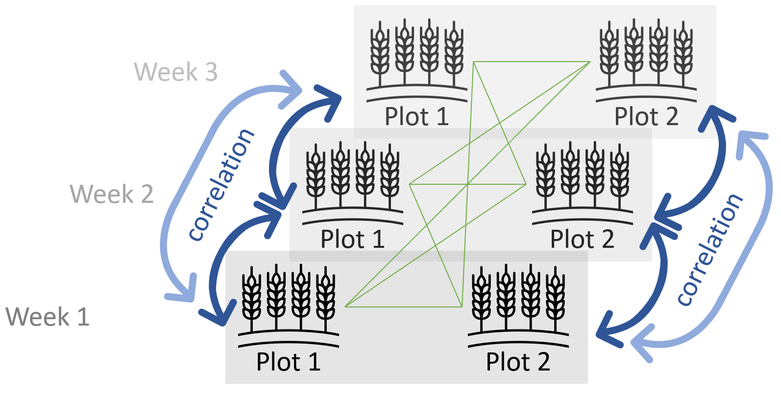
Take the visualisation on the left depicting a subset of our data. Here, you can see plots 1 and 2 (out of the total of 20 in our dataset) side by side. Furthermore, they are shown for weeks 1-3 (out of the total of 5 in our dataset). Thus, a total of six values are represented, coming from only two subjects/plots, but obtained in three different weeks. The blue arrows represent correlation among errors. For these six measurements, there are six blue arrows, since there are six error pairs that come from the same plot, respectively. The green lines on the other hand represent error pairs that do not come from the same plot and thus are assumed to be independent. Finally, notice that the errors coming from the same plot, but with two instead of just one week between their measurements, are shown in a lighter blue. This is because one may indeed assume a weaker correlation between errors that are further apart in terms of time passed between measurements.
The latter can be achieved by using a correlation structure for repeated measures over time. Maybe most popular correlation structure is called first order autoregressive AR(1). It should be noted that this correlation structure is useful, if all time points are equally spaced, which is the case here, as there is always exactly one week between consecutive time points. As can be seen in the analysis of Example 4 in Piepho & Edmondson (2018) and the corresponding Agritutorial vigniette, however, there are more options that just AR(1). Therefore, we will also try out multiple variance structures to model the serial correlation of our longitudinal data.
AR(1)
glmmTMB
To model the variance structure of our mimiced error term as first
order autoregressive, we replace the (1 | unit) from the
iid model with ar1(weekF + 0 | plot). As can
be seen, subjects are identified after the | and the
variance structure in this syntax.
Note that by adding the show_cor = TRUE argument to the
extract_vc function, we obtain two outputs: The variance
component estimates, as seen above for the iid model, as
well as the correlation matrix / variance structure for a single
plot.
mod.AR1 <- glmmTMB(formula = y ~ weekF * (variety + block) +
                     ar1(weekF + 0 | plot), # ar1 structure as random term to mimic error var
                   dispformula = ~ 0, # fix original error variance to 0
                   REML = TRUE,       # needs to be stated since default = ML
                   data = dat)

# Extract variance component estimates
# alternative: mod.ar1 %>% broom.mixed::tidy(effects = "ran_pars", scales = "vcov")
mod.AR1 %>% extract_vc(ci_scale = "var", show_cor = TRUE)
## $`Variance Components`
## # A tibble: 2 × 6
## group variance sd var_2.5 var_97.5 var_prop
## <chr> <dbl> <dbl> <dbl> <dbl> <dbl>
## 1 plot 0.022 0.149 0.013 0.038 0.2
## 2 Residual 0 0 NA NA 0
##
## $Cor
## $Cor$plot
## weekFweek1 weekFweek2 weekFweek3 weekFweek4 weekFweek5
## weekFweek1 1.000 0.749 0.561 0.420 0.315
## weekFweek2 0.749 1.000 0.749 0.561 0.420
## weekFweek3 0.561 0.749 1.000 0.749 0.561
## weekFweek4 0.420 0.561 0.749 1.000 0.749
## weekFweek5 0.315 0.420 0.561 0.749 1.000We can see that the we get \(\sigma^2_{plot} =\) 0.022 and
a \(\rho =\) 0.749.
nlme
In nlme we make use of the correlation =
argument and use the corAR1 correlation strucutre class. In its syntax, subjects
are identified after the |.
mod.AR1.nlme <- gls(model = y ~ weekF * (block + variety),
                    correlation = corAR1(form = ~ weekN | plot),
                    data = dat)

# Extract variance component estimates
tibble(varstruct = "ar(1)") %>%
  mutate(sigma    = mod.AR1.nlme$sigma,
         rho      = coef(mod.AR1.nlme$modelStruct$corStruct, unconstrained = FALSE)) %>%
  mutate(Variance = sigma^2,
         Corr1wk  = rho,
         Corr2wks = rho^2,
         Corr3wks = rho^3,
         Corr4wks = rho^4)
## # A tibble: 1 × 8
## varstruct sigma rho Variance Corr1wk Corr2wks Corr3wks Corr4wks
## <chr> <dbl> <dbl> <dbl> <dbl> <dbl> <dbl> <dbl>
## 1 ar(1) 0.149 0.749 0.0222 0.749 0.561 0.420 0.315We can see that the we get \(\sigma^2_{plot} =\) 0.022 and
a \(\rho =\) 0.749.
nlme V2
For completeness, I want to show that the same model can also be fit
in nlme via the corExp correlation strucutre class. Note that this was
actually done in the Agritutorial vigniette and Piepho & Edmondson (2018) write in Appendix 2:
“Initially, we used corCAR1() to fit the model correlation structure but
subsequently found that corExp() was more flexible as it allowed the
inclusion of a “nugget” term, which seemingly cannot be done with
corCAR1(). We note that it is essential that the variable weeks in the
specification of the correlation structure, corr = corExp (form =
~weeks|Plots), is a numeric variable with values representing the time
values of the repeated measurements. Note that this code will also work
for repeated observations that are not necessarily equally spaced. It is
also necessary that each plot has a unique level for the variable
Plots.”
Notice also that the increased flexibility comes at a price: Extracting the estimate for \(\rho\) takes quite some code:
mod.AR1.nlme.V2 <- gls(model = y ~ weekF * (variety + block),
                       correlation = corExp(form = ~ weekN | plot),
                       data = dat)

tibble(varstruct = "ar(1)") %>%
  mutate(sigma    = mod.AR1.nlme.V2$sigma,
         rho      = exp(-1/coef(mod.AR1.nlme.V2$modelStruct$corStruct,
                                unconstrained = FALSE))) %>%
  mutate(Variance = sigma^2,
         Corr1wk  = rho,
         Corr2wks = rho^2,
         Corr3wks = rho^3,
         Corr4wks = rho^4)
## # A tibble: 1 × 8
## varstruct sigma rho Variance Corr1wk Corr2wks Corr3wks Corr4wks
## <chr> <dbl> <dbl> <dbl> <dbl> <dbl> <dbl> <dbl>
## 1 ar(1) 0.149 0.749 0.0222 0.749 0.561 0.420 0.315We can see that the we get \(\sigma^2_{plot} =\) 0.022 and
a \(\rho =\) 0.749.
AR(1) + nugget
glmmTMB
not possible ?
mod.AR1nugget <- glmmTMB(formula = y ~ weekF * (variety + block) +
                           ar1(weekF + 0 | plot), # ar1 structure as random term to mimic error var
                         # dispformula = ~ 0, # error variance allowed = nugget!
                         REML = TRUE,       # needs to be stated since default = ML
                         data = dat)

# show variance components
# alternative: mod.AR1nugget %>% broom.mixed::tidy(effects = "ran_pars", scales = "vcov")
mod.AR1nugget %>% extract_vc(ci_scale = "var", show_cor = TRUE)

# We can see that the we get $\sigma^2_{plot} =$ `0.019`, an additional residual/nugget variance  $\sigma^2_{N} =$ `0.004` and a $\rho =$ of `0.908`.
nlme
As pointed out by Piepho & Edmondson (2018) write in Appendix 2: “Initially, we used corCAR1() to fit the model correlation structure but subsequently found that corExp() was more flexible as it allowed the inclusion of a “nugget” term, which seemingly cannot be done with corCAR1(). We note that it is essential that the variable weeks in the specification of the correlation structure, corr = corExp (form = ~weeks|Plots), is a numeric variable with values representing the time values of the repeated measurements. Note that this code will also work for repeated observations that are not necessarily equally spaced. It is also necessary that each plot has a unique level for the variable Plots.” This was also done in the Agritutorial vigniette.
Notice also that the increased flexibility comes at a price: Extracting the estimate for \(\rho\) takes quite some code:
mod.AR1nugget.nlme <- gls(model = y ~ weekF * (block + variety),
                          correlation = corExp(form = ~ weekN | plot, nugget = TRUE),
                          data = dat)

tibble(varstruct = "ar(1) + nugget") %>%
  mutate(sigma    = mod.AR1nugget.nlme$sigma,
         nugget   = coef(mod.AR1nugget.nlme$modelStruct$corStruct,
                         unconstrained = FALSE)[2],
         rho      = (1-coef(mod.AR1nugget.nlme$modelStruct$corStruct,
                            unconstrained = FALSE)[2])*
                    exp(-1/coef(mod.AR1nugget.nlme$modelStruct$corStruct,
                                unconstrained = FALSE)[1])) %>%
  mutate(Variance = sigma^2,
         Corr1wk  = rho,
         Corr2wks = rho^2,
         Corr3wks = rho^3,
         Corr4wks = rho^4)
## # A tibble: 1 × 9
## varstruct sigma nugget rho Variance Corr1wk Corr2wks Corr3wks Corr4wks
## <chr> <dbl> <dbl> <dbl> <dbl> <dbl> <dbl> <dbl> <dbl>
## 1 ar(1) + nugget 0.150 0.172 0.752 0.0225 0.752 0.565 0.425 0.319We can see that the we get \(\sigma^2_{plot} =\) 0.0225 and
a \(\rho =\) 0.752.
CS
glmmTMB (hCS!)
Note that glmmTMB() only allows for
heterogengeous compound symmetry and not standard compound
symmetry!
To model the variance structure of our mimiced error term as a
heterogeneous compound symmetry structure, we use
cs(weekF + 0 | plot). Notice that this is not the simple
compound symmetry structure that Piepho & Edmondson (2018) applied, because
glmmTMB() only allows for heterogeneous compound symmetry
at the moment.
mod.hCS <- glmmTMB(formula = y ~ weekF * (variety + block) +
                     cs(weekF + 0 | plot), # hcs structure as random term to mimic error var
                   dispformula = ~ 0, # fix original error variance to 0
                   REML = TRUE,       # needs to be stated since default = ML
                   data = dat)

# show variance components
# alternative: mod.hCS %>% broom.mixed::tidy(effects = "ran_pars", scales = "vcov")
mod.hCS %>% extract_vc(ci_scale = "var", show_cor = TRUE)
## $`Variance Components`
## # A tibble: 6 × 7
## group effect variance sd var_2.5 var_97.5 var_prop
## <chr> <chr> <dbl> <dbl> <dbl> <dbl> <dbl>
## 1 plot weekFweek1 0.021 0.144 0.009 0.046 0.181
## 2 plot weekFweek2 0.022 0.147 0.01 0.048 0.188
## 3 plot weekFweek3 0.021 0.146 0.01 0.047 0.186
## 4 plot weekFweek4 0.029 0.171 0.014 0.063 0.254
## 5 plot weekFweek5 0.022 0.148 0.01 0.049 0.191
## 6 Residual <NA> 0 0 NA NA 0
##
## $Cor
## $Cor$plot
## weekFweek1 weekFweek2 weekFweek3 weekFweek4 weekFweek5
## weekFweek1 1.000 0.702 0.702 0.702 0.702
## weekFweek2 0.702 1.000 0.702 0.702 0.702
## weekFweek3 0.702 0.702 1.000 0.702 0.702
## weekFweek4 0.702 0.702 0.702 1.000 0.702
## weekFweek5 0.702 0.702 0.702 0.702 1.000We can see that the we get heterogeneous \(\sigma^2_{plot}\) estimates per week:
0.021, 0.022, 0.021,
0.029, 0.022 and a \(\rho =\) 0.702.
nlme
In nlme we make use of the correlation =
argument and use the corCompSymm correlation strucutre class. In its syntax, subjects
are identified after the |.
mod.CS.nlme <- gls(y ~ weekF * (block + variety),
                   corr = corCompSymm(form = ~ weekN | plot),
                   data = dat)

tibble(varstruct = "cs") %>%
  mutate(sigma    = mod.CS.nlme$sigma,
         rho      = coef(mod.CS.nlme$modelStruct$corStruct, unconstrained = FALSE)) %>%
  mutate(Variance = sigma^2,
         Corr1wk  = rho,
         Corr2wks = rho,
         Corr3wks = rho,
         Corr4wks = rho)
## # A tibble: 1 × 8
## varstruct sigma rho Variance Corr1wk Corr2wks Corr3wks Corr4wks
## <chr> <dbl> <dbl> <dbl> <dbl> <dbl> <dbl> <dbl>
## 1 cs 0.152 0.701 0.0232 0.701 0.701 0.701 0.701We can see that the we get \(\sigma^2_{plot} =\) 0.023 and
a \(\rho =\) of 0.701.
Toeplitz
glmmTMB
To model the variance structure of our mimiced error term as a
toeplitz structure, we use toep(weekF + 0 | plot).
mod.Toep <- glmmTMB(formula = y ~ weekF * (variety + block) +
                     toep(weekF + 0 | plot), # teop structure as random term to mimic err var
                   dispformula = ~ 0, # fix original error variance to 0
                   REML = TRUE,       # needs to be stated since default = ML
                   data = dat)

# show variance components
# alternative: mod.Toep %>% broom.mixed::tidy(effects = "ran_pars", scales = "vcov")
mod.Toep %>% extract_vc(ci_scale = "var", show_cor = TRUE)
## $`Variance Components`
## # A tibble: 6 × 7
## group effect variance sd var_2.5 var_97.5 var_prop
## <chr> <chr> <dbl> <dbl> <dbl> <dbl> <dbl>
## 1 plot weekFweek1 0.021 0.144 0.009 0.046 0.182
## 2 plot weekFweek2 0.023 0.152 0.01 0.052 0.202
## 3 plot weekFweek3 0.022 0.147 0.01 0.048 0.19
## 4 plot weekFweek4 0.029 0.17 0.013 0.062 0.253
## 5 plot weekFweek5 0.02 0.141 0.009 0.043 0.174
## 6 Residual <NA> 0 0 NA NA 0
##
## $Cor
## $Cor$plot
## weekFweek1 weekFweek2 weekFweek3 weekFweek4 weekFweek5
## weekFweek1 1.000 0.764 0.691 0.637 0.552
## weekFweek2 0.764 1.000 0.764 0.691 0.637
## weekFweek3 0.691 0.764 1.000 0.764 0.691
## weekFweek4 0.637 0.691 0.764 1.000 0.764
## weekFweek5 0.552 0.637 0.691 0.764 1.000We can see that the we get heterogeneous \(\sigma^2_{plot}\) estimates per week:
0.021, 0.023, 0.022,
0.029, 0.020 and a heterogeneous \(\rho\) per week-difference:
0.764, 0.691, 0.637 and
0.552.
nlme
not possible? At least it is not included in the agriTutorial vigniette and there is no obviously corresponding cor.class found in the nlme documentation.
UN
glmmTMB
To model the variance structure of our mimiced error term as a
completely unstrucutred variance structure, we use
us(weekF + 0 | plot).
mod.UN <- glmmTMB(formula = y ~ weekF * (variety + block) +
                     us(weekF + 0 | plot), # us structure as random term to mimic error var
                   dispformula = ~ 0, # fix original error variance to 0
                   REML = TRUE,       # needs to be stated since default = ML
                   data = dat)

# show variance components
# alternative: mod.UN %>% broom.mixed::tidy(effects = "ran_pars", scales = "vcov")
mod.UN %>% extract_vc(ci_scale = "var", show_cor = TRUE)
## $`Variance Components`
## # A tibble: 6 × 7
## group effect variance sd var_2.5 var_97.5 var_prop
## <chr> <chr> <dbl> <dbl> <dbl> <dbl> <dbl>
## 1 plot weekFweek1 0.02 0.141 0.009 0.044 0.17
## 2 plot weekFweek2 0.021 0.143 0.009 0.046 0.177
## 3 plot weekFweek3 0.022 0.149 0.01 0.05 0.192
## 4 plot weekFweek4 0.033 0.181 0.015 0.073 0.282
## 5 plot weekFweek5 0.021 0.143 0.009 0.046 0.178
## 6 Residual <NA> 0 0 NA NA 0
##
## $Cor
## $Cor$plot
## weekFweek1 weekFweek2 weekFweek3 weekFweek4 weekFweek5
## weekFweek1 1.000 0.708 0.644 0.748 0.534
## weekFweek2 0.708 1.000 0.634 0.744 0.549
## weekFweek3 0.644 0.634 1.000 0.934 0.718
## weekFweek4 0.748 0.744 0.934 1.000 0.776
## weekFweek5 0.534 0.549 0.718 0.776 1.000As can be seen, each week gets its own variance and also each pair of weeks gets individual correlations.
nlme
In nlme we make use of the correlation =
argument and use the corSymm correlation strucutre class in combination with the
varIdent() in the weights= argument, which is used to
allow for different variances according to the levels of a
classification factor. In its syntax, subjects are identified after
the |.
mod.UN.nlme <- gls(y ~ weekF * (block + variety),
                   corr = corSymm(form = ~ 1 | plot),
                   weights = varIdent(form = ~ 1|weekF),
                   data = dat)

# Extract variance component estimates: variances
mod.UN.nlme$modelStruct$varStruct %>%
  coef(unconstrained = FALSE, allCoef = TRUE) %>%
  enframe(name = "grp", value = "varStruct") %>%
  mutate(sigma         = mod.UN.nlme$sigma) %>%
  mutate(StandardError = sigma * varStruct) %>%
  mutate(Variance      = StandardError ^ 2)
## # A tibble: 5 × 5
## grp varStruct sigma StandardError Variance
## <chr> <dbl> <dbl> <dbl> <dbl>
## 1 week1 1 0.141 0.141 0.0197
## 2 week2 1.02 0.141 0.143 0.0206
## 3 week3 1.06 0.141 0.149 0.0223
## 4 week4 1.29 0.141 0.181 0.0327
## 5 week5 1.02 0.141 0.143 0.0206# Extract variance component estimates: correlations
mod.UN.nlme$modelStruct$corStruct## Correlation structure of class corSymm representing
## Correlation:
## 1 2 3 4
## 2 0.708
## 3 0.644 0.634
## 4 0.748 0.744 0.934
## 5 0.534 0.549 0.718 0.776As can be seen, each week gets its own variance and also each pair of weeks gets individual correlations.
Model selection
variance structure
glmmTMB
In order to select the best model here, we can simply compare their AIC values, since all models are identical regarding their fixed effects part. The smaller the value of AIC, the better is the fit:
AICcmodavg::aictab(
  cand.set = list(mod.iid, mod.hCS, mod.AR1, mod.Toep, mod.UN),
  modnames = c("iid", "hCS", "AR1", "Toeplitz", "UN"),
  second.ord = FALSE) # get AIC instead of AICc
##
## Model selection based on AIC:
##
## K AIC Delta_AIC AICWt Cum.Wt LL
## AR1 42 38.04 0.00 0.96 0.96 22.98
## hCS 46 45.25 7.20 0.03 0.98 23.38
## UN 55 47.10 9.05 0.01 0.99 31.45
## Toeplitz 49 47.88 9.84 0.01 1.00 25.06
## iid 41 78.26 40.22 0.00 1.00 1.87According to the AIC value, the mod.AR1 model is the
best, suggesting that the plot values across weeks are indeed
autocorrelated (as opposed to the mod.iid model) and that
from all the potential variance structures, the first order
autoregressive structure was best able to capture this
autocorrelation.
nlme
In order to select the best model here, we can simply compare their AIC values, since all models are identical regarding their fixed effects part. The smaller the value of AIC, the better is the fit:
AICcmodavg::aictab(
  cand.set = list(mod.iid.nlme, mod.CS.nlme, mod.AR1.nlme, mod.AR1nugget.nlme, mod.UN.nlme),
  modnames = c("iid", "CS", "AR1", "AR1 + nugget", "UN"),
  second.ord = FALSE) # get AIC instead of AICc
##
## Model selection based on AIC:
##
## K AIC Delta_AIC AICWt Cum.Wt Res.LL
## AR1 + nugget 43 37.48 0.00 0.42 0.42 24.26
## AR1 42 38.04 0.57 0.31 0.73 22.98
## CS 42 38.38 0.90 0.27 1.00 22.81
## UN 55 47.10 9.62 0.00 1.00 31.45
## iid 41 78.26 40.78 0.00 1.00 1.87According to the AIC value, the mod.AR1 model is the
best, suggesting that the plot values across weeks are indeed
autocorrelated (as opposed to the mod.iid model) and that
from all the potential variance structures, the first order
autoregressive structure was best able to capture this
autocorrelation.
time trend as (polynomial) regression model
So far, we have focussed on dealing with potentially correlated error terms for our repeated measures data. Now that we dealt with this and found an optimal solution, we are now ready to select a regression model for time trend. As a reminder, this is the data we are dealing with (this time not animated):
ggplot(data = dat,
       aes(y = y, x = weekF,
           group = variety,
           color = variety)) +
  geom_point(alpha = 0.75, size = 3) +
  stat_summary(fun=mean, geom="line") + # lines between means
  scale_y_continuous(
    name = "Leaf area index",
    limits = c(0, 6.5),
    expand = c(0, 0),
    breaks = c(0:6)) +
  scale_color_manual(values = var_colors) +
  theme_bw() +
  theme(legend.position = "bottom",
        axis.title.x = element_blank())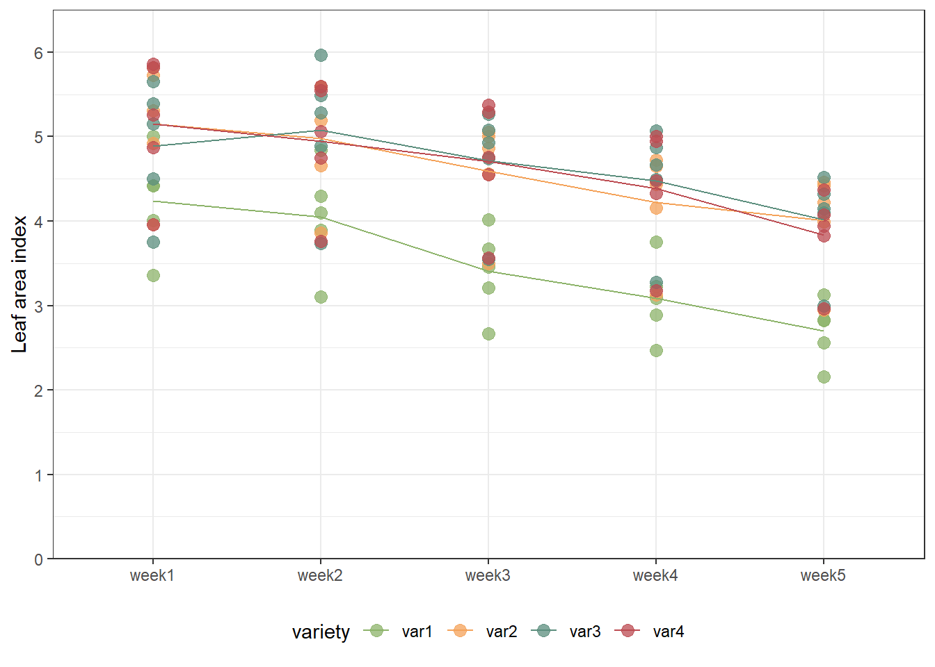
It can now be asked whether the trend over time is simply linear (in
the sense of y = a + bx) or can better be modelled as with
a polynomial regression (i.e. y = a + bx + cx² or
y = a + bx + cx² + dx³ and so on). Very roughly put, we are
asking whether a straight line fits the data well enough or if we should
instead use a model that results in some sort of curved line.
In order to answer this question, we use the lack-of-fit method to determine which degree of a polynomial regression we should go with. We start with the linear regression model.
work in progress
Please feel free to contact me about any of this!
schmidtpaul1989@outlook.com