Heterogeneous error variance

# packages
pacman::p_load(conflicted, # package function conflicts
               dplyr, purrr, stringr, tibble, tidyr, # data handling
               nlme, lme4, glmmTMB, sommer, # mixed modelling
               AICcmodavg, broom.mixed)     # mixed model extractions

# package function conflicts
conflict_prefer("filter", "dplyr")

# data
dat <- agridat::mcconway.turnip %>%
  as_tibble() %>%
  mutate(densf = density %>% as.factor)

gen	date	density	block	yield	densf
Barkant	21Aug1990	1	B1	2.7	1
Barkant	21Aug1990	1	B2	1.4	1
Barkant	21Aug1990	1	B3	1.2	1
Barkant	21Aug1990	1	B4	3.8	1
Barkant	21Aug1990	2	B1	7.3	2
Barkant	21Aug1990	2	B2	3.8	2
Barkant	21Aug1990	2	B3	3.0	2
Barkant	21Aug1990	2	B4	1.2	2
Barkant	21Aug1990	4	B1	6.5	4
Barkant	21Aug1990	4	B2	4.6	4
Barkant	21Aug1990	4	B3	4.7	4
Barkant	21Aug1990	4	B4	0.8	4
Barkant	21Aug1990	8	B1	8.2	8
Barkant	21Aug1990	8	B2	4.0	8
Barkant	21Aug1990	8	B3	6.0	8
Barkant	21Aug1990	8	B4	2.5	8
Barkant	28Aug1990	1	B1	4.4	1
Barkant	28Aug1990	1	B2	0.4	1
Barkant	28Aug1990	1	B3	6.5	1
Barkant	28Aug1990	1	B4	3.1	1
Barkant	28Aug1990	2	B1	2.6	2
Barkant	28Aug1990	2	B2	7.1	2
Barkant	28Aug1990	2	B3	7.0	2
Barkant	28Aug1990	2	B4	3.2	2
Barkant	28Aug1990	4	B1	24.0	4
Barkant	28Aug1990	4	B2	14.9	4
Barkant	28Aug1990	4	B3	14.6	4
Barkant	28Aug1990	4	B4	2.6	4
Barkant	28Aug1990	8	B1	12.2	8
Barkant	28Aug1990	8	B2	18.9	8
Barkant	28Aug1990	8	B3	15.6	8
Barkant	28Aug1990	8	B4	9.9	8
Marco	21Aug1990	1	B1	1.2	1
Marco	21Aug1990	1	B2	1.3	1
Marco	21Aug1990	1	B3	1.5	1
Marco	21Aug1990	1	B4	1.0	1
Marco	21Aug1990	2	B1	2.2	2
Marco	21Aug1990	2	B2	2.0	2
Marco	21Aug1990	2	B3	2.1	2
Marco	21Aug1990	2	B4	2.5	2
Marco	21Aug1990	4	B1	2.2	4
Marco	21Aug1990	4	B2	6.2	4
Marco	21Aug1990	4	B3	5.7	4
Marco	21Aug1990	4	B4	0.6	4
Marco	21Aug1990	8	B1	4.0	8
Marco	21Aug1990	8	B2	2.8	8
Marco	21Aug1990	8	B3	10.8	8
Marco	21Aug1990	8	B4	3.1	8
Marco	28Aug1990	1	B1	2.5	1
Marco	28Aug1990	1	B2	1.6	1
Marco	28Aug1990	1	B3	1.3	1
Marco	28Aug1990	1	B4	0.3	1
Marco	28Aug1990	2	B1	5.5	2
Marco	28Aug1990	2	B2	1.2	2
Marco	28Aug1990	2	B3	2.0	2
Marco	28Aug1990	2	B4	0.9	2
Marco	28Aug1990	4	B1	4.7	4
Marco	28Aug1990	4	B2	13.2	4
Marco	28Aug1990	4	B3	9.0	4
Marco	28Aug1990	4	B4	2.9	4
Marco	28Aug1990	8	B1	14.9	8
Marco	28Aug1990	8	B2	13.3	8
Marco	28Aug1990	8	B3	9.3	8
Marco	28Aug1990	8	B4	3.6	8

Motivation

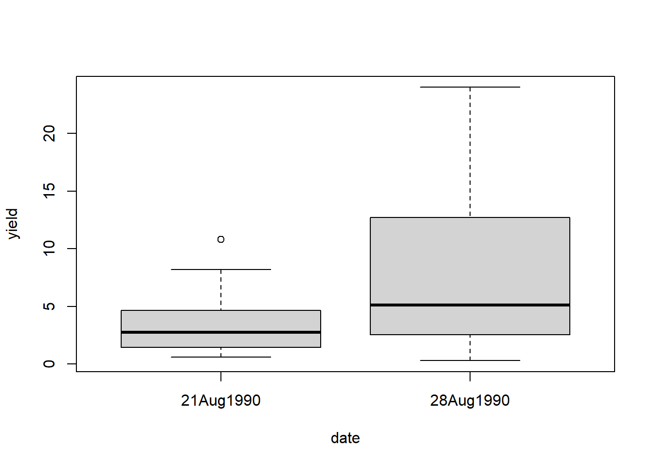
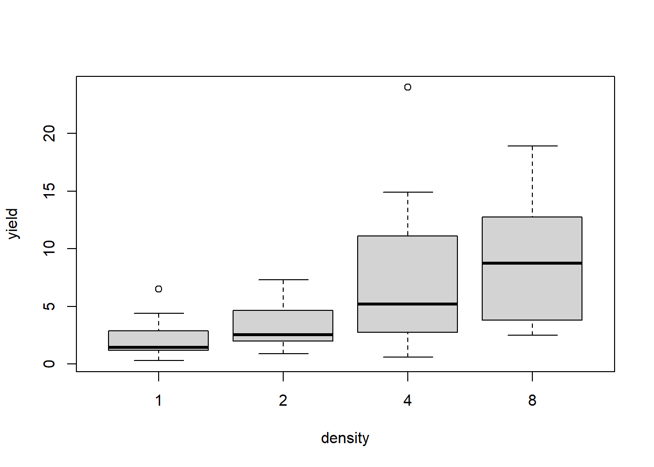
This is a randomized complete block design (4 blocks) with three treatment factors: genotype, date and density, leading to 16 treatment level combinations (2 genotypes, 2 planting dates, 4 densities) (Piepho, 2009). It can be argued that heterogeneous error variances (i.e. heteroscedasticity) for two of the treatments should be considered:

boxplot(yield ~ date, data = dat)

boxplot(yield ~ density, data = dat)

5 Models

We therefore set up 5 models, which only differ in the variance structure in the error term. More specifically, we allow for different heterogeneous error variances / heteroscedascity per group for the effect levels of Date and Density. This type of variance structure is sometimes also referred to as diagonal.

Regarding the effects in the model, we take the same approach as Piepho (2009), which calls for fixed main effects for gen, date and densf as well as all their interaction effects, plus random block effects.

The different variance structures in the error term of the 5 models are summarised in the table below (only mods 1-4 can be found in Piepho (2009)). Further notice the difference between mod4 and mod5: mod4 includes the direct product (a.k.a. Kronecker product) structure of the two diag-structures of Date and Density. mod5 simply includes a diag-structure for the Date-Density-combinations (see our summary on variance structures for more info).

	Term in multiplicative variance structure				Number of variance
Model	Block	Genotype	Date	Density	parametersa	estimatesa
mod1	Identity	Identity	Identity	Identity	1	1
mod2	Identity	Identity	Identity	Diagonal	2	2
mod3	Identity	Identity	Diagonal	Identity	4	4
mod4	Identity	Identity	Diagonal	Diagonal	5	8
mod5	Identity	Identity	Diag-	onal	8	8
a ignoring the random block effects

nlme

To obtain heterogeneous variances in nlme, we need to use the variance function varIdent() in the weights= argument, which is used to allow for different variances according to the levels of a classification factor. For the multiplicative variance structure in mod4, we can combine two variance functions via varComb(). Since it is not possible to pass an interaction term to the varIdent() function as varIdent(form=~1|date:densf), we must manually create a column that combines the two columns in order to fit mod5:

dat <- dat %>%
  mutate(date_densf = interaction(date, densf)) # needed for mod5

mod1.nlme <- nlme::lme(fixed   = yield ~ gen * date * densf,  
                       random  = ~ 1 | block, 
                       weights = NULL, # default, i.e. homoscedastic errors
                       data    = dat)

mod2.nlme <- mod1.nlme %>%
  update(weights = varIdent(form =  ~ 1 | date))

mod3.nlme <- mod1.nlme %>%
  update(weights = varIdent(form =  ~ 1 | densf))

mod4.nlme <- mod1.nlme %>%
  update(weights = varComb(varIdent(form =  ~ 1 | date),
                           varIdent(form =  ~ 1 | densf))) 

mod5.nlme <- mod1.nlme %>%
  update(weights = varIdent(form =  ~ 1 | date_densf))

lme4

The short answer here is that with lme4 it is not possible to fit any variance structures, so that in this chapter only mod1 could be modeled:

mod1.lme4 <- lmer(formula = yield ~ gen * date * densf + (1 | block),
                  data    = dat)

# mod2.lme4 - not possible

# mod3.lme4 - not possible

# mod4.lme4 - not possible

# mod5.lme4 - not possible

More specifically, we can read in an lme4 vigniette: “The main advantage of nlme relative to lme4 is a user interface for fitting models with structure in the residuals (various forms of heteroscedasticity and autocorrelation) and in the random-effects covariance matrices (e.g., compound symmetric models). With some extra effort, the computational machinery of lme4 can be used to fit structured models that the basic lmer function cannot handle (see Appendix A)”

Michael Clark puts it as “Unfortunately, lme4 does not provide the ability to model the residual covariance structure, at least not in a straightforward fashion”

Thus, there is no info on this package for this chapter beyond this point, except for model 1.

glmmTMB

In glmmTMB() it is -to our knowledge- not possible to adjust the variance structure of the error.

Just like in nlme, there is a weights= argument in glmmTMB(). However, to our understanding, they have different functions:

In nlme, it requires “an optional varFunc object or one-sided formula describing the within-group heteroscedasticity structure” (nlme RefMan) and we make use of this in the chapter at hand.

In glmmTMB, the RefMan only states “weights, as in glm. Not automatically scaled to have sum 1”. Following this trail, the glm documentation description for the weights= argument is “an optional vector of ‘prior weights’ to be used in the fitting process. Should be NULL or a numeric vector.”. Accordingly, it cannot be used to allow for heterogeneous error variances in this package.

We can, however, “fix the residual variance to be 0 (actually a small non-zero value)” and therefore “force variance into the random effects” (glmmTMB RefMan) via adding the dispformula = ~ 0 argument. Thus, when doing so, we need to make sure to also add a random term to the model with the desired variance structure. By taking both of these actions, we are essentially mimicing the error (variance) as a random effect (variance). We achieve this by first creating a unit column in the data with different entries for each data point:

dat <- dat %>%
  mutate(unit = 1:n() %>% as.factor) # new column with running number

We should now be able to mimic the error variance via the random term (1|unit). We can verify this quickly, by modelling mod1 with a homoscedastic error variance in the standard fashion (mod1) and via a mimicked error term (mod1b). For all other models we make use of the diag() function. Notice that we must write diag(TERM + 0|unit), since leaving out the + 0 would by default lead to estimating not only the desired heterogeneous variances, but an additional overall variance.

Notice that at the moment, it is not possible to fit mod4 with glmmTMB.

mod1.glmm <- glmmTMB(formula = yield ~ gen * date * densf + (1 | block), 
                     dispformula = ~ 1,  # = default i.e. homoscedastic error variance
                     REML = TRUE,        # needs to be stated since default = ML
                     data = dat) 

mod1b.glmm <- mod1.glmm %>%
  update(. ~ . + (1 | unit), # add random term to mimic homoscedastic error variance
         dispformula = ~ 0) # fix original error variance to 0

mod2.glmm <- mod1.glmm %>% 
  update(. ~ . + diag(date + 0 | unit), dispformula = ~ 0)

mod3.glmm <- mod1.glmm %>% 
  update(. ~ . + diag(densf + 0 | unit), dispformula = ~ 0)

# mod4/multiplicative variance structure not possible.

mod5.glmm <- mod1.glmm %>% 
  update(. ~ . + diag(date:densf + 0 | unit), dispformula = ~ 0)

As can be seen below, mimicing the error (variance) worked, as it leads to comparable variance component estimates:

mod1.glmm %>% VarCorr()

## 
## Conditional model:
##  Groups   Name        Std.Dev.
##  block    (Intercept) 1.6768  
##  Residual             3.0970

mod1b.glmm %>% VarCorr()

## 
## Conditional model:
##  Groups Name        Std.Dev.
##  block  (Intercept) 1.6764  
##  unit   (Intercept) 3.0970

sommer

To allow for different variance structures in the error term in sommer, we need to use the vs() function in the rcov= argument. More specifically, we need the ds() function to obtain heterogeneous variances.

mod1.somm <- mmer(fixed  = yield ~ gen * date * densf, 
                  random = ~ block,
                  rcov   = ~ units, # default
                  data   = dat, verbose=F)

mod2.somm <- mmer(fixed  = yield ~ gen * date * densf, 
                  random = ~ block,
                  rcov   = ~ vs(ds(date), units), 
                  data   = dat, verbose=F)

mod3.somm <- mmer(fixed  = yield ~ gen * date * densf, 
                  random = ~ block,
                  rcov   = ~ vs(ds(densf), units), 
                  data   = dat, verbose=F)

mod4.somm <- mmer(fixed  = yield ~ gen * date * densf, 
                  random = ~ block,
                  rcov   = ~ vs(ds(date), units) + vs(ds(densf), units), 
                  data   = dat, verbose=F)

mod5.somm <- mmer(fixed  = yield ~ gen * date * densf, 
                  random = ~ block,
                  rcov   = ~ vs(ds(date), ds(densf), units), 
                  data   = dat, verbose=F)

SAS

/* mod1 */ proc mixed data=dat; class gen date densf block; model yield = gen * date * densf; random block; ods output covparms=mod1sasVC FitStatistics=mod1sasAIC; run; /* mod2 */ proc mixed data=dat; class gen date densf block; model yield = gen * date * densf; random block; repeated / group=date; ods output covparms=mod2sasVC FitStatistics=mod2sasAIC; run; /* mod3 */ proc mixed data=dat; class gen date densf block; model yield = gen * date * densf; random block; repeated / group=densf; ods output covparms=mod3sasVC FitStatistics=mod3sasAIC; run; /* mod4 */ proc mixed data=dat; class gen date densf block; model yield = gen * date * densf; random block; repeated / local=exp(date densf); ods output covparms=mod4sasVC FitStatistics=mod4sasAIC; run; /* mod5 */ proc mixed data=dat; class gen date densf block; model yield = gen * date * densf; random block; repeated / group=date*densf; ods output covparms=mod5sasVC FitStatistics=mod5sasAIC; run;

Variance Component Extraction

After fitting the models, we would now like to extract the variance component estimates.

nlme

As far as we know, it is quite cumbersome to extract variance component estimates from nlme objects (in a table format we are used to), even with helper packages such as broom.mixed (see github issue ). Beneath is the the most elegant approach we have so far when trying to get similarly formatted output for all 5 models. The general approach is to first get a table with a column for

• all levels / level-combinations for which heterogeneous error variances were fit
• their respective value of the model-object’s varStruct and
• the overall value of the model-object’s sigma (= standard deviation for error term).

By multiplying the latter two, we receive the respective standard error estimate, which needs to be squared in order to obtain the respective variance component estimate.

mod1

mod1.nlme.VC <- tibble(grp = "homoscedastic", varStruct = 1) %>% 
  mutate(sigma         = mod1.nlme$sigma) %>% 
  mutate(StandardError = sigma*varStruct) %>% 
  mutate(Variance      = StandardError^2)

grp	varStruct	sigma	StandardError	Variance
homoscedastic	1	3.097	3.097	9.591

mod2

mod2.nlme.VC <- mod2.nlme$modelStruct$varStruct %>%
  coef(unconstrained = FALSE, allCoef = TRUE) %>%
  enframe(name = "grp", value = "varStruct") %>%
  mutate(sigma         = mod2.nlme$sigma) %>%
  mutate(StandardError = sigma * varStruct) %>%
  mutate(Variance      = StandardError ^ 2)

grp	varStruct	sigma	StandardError	Variance
21Aug1990	1.000	2.075	2.075	4.306
28Aug1990	1.898	2.075	3.938	15.505

mod3

mod3.nlme.VC <- mod3.nlme$modelStruct$varStruct %>%
  coef(unconstrained = FALSE, allCoef = TRUE) %>%
  enframe(name = "grp", value = "varStruct") %>%
  mutate(sigma         = mod3.nlme$sigma) %>%
  mutate(StandardError = sigma * varStruct) %>%
  mutate(Variance      = StandardError ^ 2)

grp	varStruct	sigma	StandardError	Variance
1	1.000	1.501	1.501	2.252
2	1.276	1.501	1.916	3.670
4	3.334	1.501	5.004	25.037
8	2.434	1.501	3.652	13.339

mod4

mod4.nlme.varStruct.A <- mod4.nlme$modelStruct$varStruct$A %>%
  coef(unconstrained = FALSE, allCoef = TRUE) %>%
  enframe(name = "grpA", value = "varStructA")

mod4.nlme.varStruct.B <- mod4.nlme$modelStruct$varStruct$B %>%
  coef(unconstrained = FALSE, allCoef = TRUE) %>%
  enframe(name = "grpB", value = "varStructB")

mod4.nlme.VC <- expand.grid(mod4.nlme.varStruct.A$grpA,
                            mod4.nlme.varStruct.B$grpB,
                            stringsAsFactors = FALSE) %>%
  rename(grpA = Var1, grpB = Var2) %>%
  left_join(x = ., y = mod4.nlme.varStruct.A, by = "grpA") %>%
  left_join(x = ., y = mod4.nlme.varStruct.B, by = "grpB") %>%
  mutate(sigma         = mod4.nlme$sigma) %>%
  mutate(StandardError = sigma * varStructA * varStructB) %>%
  mutate(Variance      = StandardError ^ 2)

grpA	grpB	varStructA	varStructB	sigma	StandardError	Variance
21Aug1990	1	1.000	1.000	1.015	1.015	1.030
21Aug1990	2	1.000	1.482	1.015	1.503	2.260
21Aug1990	4	1.000	3.237	1.015	3.285	10.790
21Aug1990	8	1.000	2.772	1.015	2.813	7.910
28Aug1990	1	1.747	1.000	1.015	1.773	3.143
28Aug1990	2	1.747	1.482	1.015	2.627	6.900
28Aug1990	4	1.747	3.237	1.015	5.740	32.945
28Aug1990	8	1.747	2.772	1.015	4.914	24.151

mod5

mod5.nlme.VC <- mod5.nlme$modelStruct$varStruct %>%
  coef(unconstrained = FALSE, allCoef = TRUE) %>%
  enframe(name = "grp", value = "varStruct") %>%
  separate(grp, sep = "[.]", into = c("grpA", "grpB")) %>%
  mutate(sigma         = mod5.nlme$sigma) %>%
  mutate(StandardError = sigma * varStruct) %>%
  mutate(Variance      = StandardError ^ 2)

grpA	grpB	varStruct	sigma	StandardError	Variance
21Aug1990	1	1.000	0.938	0.938	0.880
21Aug1990	2	1.872	0.938	1.755	3.081
21Aug1990	4	2.668	0.938	2.502	6.262
21Aug1990	8	3.331	0.938	3.124	9.760
28Aug1990	1	1.979	0.938	1.856	3.446
28Aug1990	2	2.383	0.938	2.235	4.997
28Aug1990	4	7.394	0.938	6.935	48.095
28Aug1990	8	4.761	0.938	4.465	19.938

We want to point out that the tidy(effects="ran_pars") function of the broom.mixed package (which we used it in this chapter to obtain the variance component estimates from glmmTMB() models) actually works on lme() objects as well (but it does not on gls() and nlme()). We did not use it here, however, since it only seems to provide the sigma estimate and not the varStruct estimates (see github issue).

lme4

In order to extract variance component estimates from lme4 objects (in a table format we are used to), we here use the tidy() function from the helper package broom.mixed:

mod1

mod1.lme4.VC <- mod1.lme4 %>%
  tidy(effects = "ran_pars", scales = "vcov") %>%
  separate(term, sep = "__", into = c("term", "grp")) %>%
  filter(group == "Residual")

effect	group	term	grp	estimate
ran_pars	Residual	var	Observation	9.591

glmmTMB

In order to extract variance component estimates from glmmTMB objects (in a table format we are used to), we here use the tidy() function from the helper package broom.mixed:

mod1

mod1.glmm.VC <- mod1.glmm %>%
  tidy(effects = "ran_pars", scales = "vcov") %>%
  separate(term, sep = "__", into = c("term", "grp")) %>%
  filter(group == "Residual")

effect	component	group	term	grp	estimate
ran_pars	cond	Residual	var	Observation	9.591

mod2

mod2.glmm.VC <- mod2.glmm %>%
  tidy(effects = "ran_pars", scales = "vcov") %>%
  separate(term, sep = "__", into = c("term", "grp")) %>%
  filter(group == "unit", term == "var")

effect	component	group	term	grp	estimate
ran_pars	cond	unit	var	date21Aug1990	4.306
ran_pars	cond	unit	var	date28Aug1990	15.505

mod3

mod3.glmm.VC <- mod3.glmm %>%
  tidy(effects = "ran_pars", scales = "vcov") %>%
  separate(term, sep = "__", into = c("term", "grp")) %>%
  filter(group == "unit", term == "var")

effect	component	group	term	grp	estimate
ran_pars	cond	unit	var	densf1	2.252
ran_pars	cond	unit	var	densf2	3.669
ran_pars	cond	unit	var	densf4	25.037
ran_pars	cond	unit	var	densf8	13.338

mod4

mod4/multiplicative variance structure not possible.

mod5

mod5.glmm.VC <- mod5.glmm %>%
  tidy(effects = "ran_pars", scales = "vcov") %>%
  separate(term, sep = "__", into = c("term", "grp")) %>%
  filter(group == "unit", term == "var") %>%
  separate(grp, sep = ":", into = c("grpA", "grpB"))

effect	component	group	term	grpA	grpB	estimate
ran_pars	cond	unit	var	date21Aug1990	densf1	0.880
ran_pars	cond	unit	var	date28Aug1990	densf1	3.446
ran_pars	cond	unit	var	date21Aug1990	densf2	3.080
ran_pars	cond	unit	var	date28Aug1990	densf2	4.997
ran_pars	cond	unit	var	date21Aug1990	densf4	6.261
ran_pars	cond	unit	var	date28Aug1990	densf4	48.089
ran_pars	cond	unit	var	date21Aug1990	densf8	9.758
ran_pars	cond	unit	var	date28Aug1990	densf8	19.936

sommer

It is quite easy to extract variance component estimates from sommer objects in a table format we are used to:

mod1

mod1.somm.VC <- summary(mod1.somm)$varcomp 

grp	VarComp	VarCompSE	Zratio	Constraint
units	9.591	2.022	4.743	Positive

mod2

mod2.somm.VC <- summary(mod2.somm)$varcomp

grp	VarComp	VarCompSE	Zratio	Constraint
21Aug1990:units	4.307	1.319	3.265	Positive
28Aug1990:units	15.499	4.560	3.399	Positive

mod3

mod3.somm.VC <- summary(mod3.somm)$varcomp

grp	VarComp	VarCompSE	Zratio	Constraint
1:units	2.256	1.000	2.257	Positive
2:units	3.668	1.573	2.332	Positive
4:units	25.013	10.275	2.434	Positive
8:units	13.323	5.507	2.419	Positive

mod4

mod4/multiplicative variance structure possible? in progress.

mod5

mod5.somm.VC <- summary(mod5.somm)$varcomp

grp	VarComp	VarCompSE	Zratio	Constraint
21Aug1990:1:units	1.016	0.665	1.528	Positive
21Aug1990:2:units	2.941	1.749	1.681	Positive
21Aug1990:4:units	5.985	3.496	1.712	Positive
21Aug1990:8:units	9.384	5.453	1.721	Positive
28Aug1990:1:units	3.298	1.955	1.687	Positive
28Aug1990:2:units	4.874	2.864	1.702	Positive
28Aug1990:4:units	47.166	27.233	1.732	Positive
28Aug1990:8:units	19.466	11.265	1.728	Positive

SAS

Thanks to the ODS (Output Delivery System) in SAS, there are no extra steps required to extract the variance component estimates. This was already achieved via the ods output covparms=modsasVC; lines in the PROC MIXED statements in the previous section. It should be noted, however, that the estimates for mod4 do need further formatting in order to obtain the here presented results. These steps are somewhat similar to those for the nlme.VC.

mod1

CovParm	Group	Estimate
Residual	homoscedastic	9.591

mod2

CovParm	Group	Estimate
Residual	date 21AUG1990	4.306
Residual	date 28AUG1990	15.505

mod3

CovParm	Group	Estimate
Residual	densf 1	2.252
Residual	densf 2	3.670
Residual	densf 4	25.037
Residual	densf 8	13.338

mod4

grpA	grpB	EXPdate	EXPdensf	sigma	Variance
21Aug1990	1	-0.558	-1.294	6.559	1.030
28Aug1990	1	0.558	-1.294	6.559	3.143
21Aug1990	2	-0.558	-0.507	6.559	2.260
28Aug1990	2	0.558	-0.507	6.559	6.900
21Aug1990	4	-0.558	1.056	6.559	10.791
28Aug1990	4	0.558	1.056	6.559	32.946
21Aug1990	8	-0.558	0.737	6.559	7.844
28Aug1990	8	0.558	0.737	6.559	23.950

mod5

CovParm	grpA	grpB	Estimate
Residual	21Aug1990	1	0.880
Residual	21Aug1990	2	3.081
Residual	21Aug1990	4	6.263
Residual	21Aug1990	8	9.760
Residual	28Aug1990	1	3.446
Residual	28Aug1990	2	4.997
Residual	28Aug1990	4	48.095
Residual	28Aug1990	8	19.938

Model Fit

As is standard procedure, we can do a model selection based on goodness-of-fit statistics such as the AIC (Akaike information criterion). In order to have a direct comparison to Table 1 in (Piepho, 2009), we also calculated the deviance (i.e. -2*loglikelihood) for each model.

For nlme, lme4 and glmmTMB, we make use of the aictab() function from the helper package AICcmodavg.

nlme

AIC.nlme <- aictab(list(mod1.nlme, mod2.nlme, mod3.nlme, mod4.nlme, mod5.nlme)) %>%
  mutate(Deviance = -2 * Res.LL) # compute deviance manually

Modnames	K	AICc	Delta_AICc	Res.LL	Deviance
Mod4	22	318.9	0.0	-125.1	250.3
Mod2	19	319.2	0.3	-132.0	263.9
Mod3	21	320.3	1.4	-128.2	256.3
Mod1	18	323.3	4.4	-136.1	272.1
Mod5	25	332.4	13.5	-124.1	248.2

lme4

AIC.lme4 <- aictab(list(mod1.lme4)) %>% # Mods 2-5 are missing
  mutate(Deviance = -2 * Res.LL) # compute deviance manually

Modnames	K	AICc	Delta_AICc	Res.LL	Deviance
Mod1	18	323.3	0	-136.1	272.1

glmmTMB

AIC.glmm <- aictab(list(mod1.glmm, mod2.glmm, mod3.glmm, mod5.glmm), 
                   modnames=c("Mod1","Mod2","Mod3","Mod5")) %>% # Mod4 is missing
  mutate(Deviance = -2*LL) # compute deviance manually

Modnames	K	AICc	Delta_AICc	LL	Deviance
Mod2	19	319.2	0.0	-132.0	263.9
Mod3	21	320.3	1.1	-128.2	256.3
Mod1	18	323.3	4.1	-136.1	272.1
Mod5	25	332.4	13.2	-124.1	248.2

sommer

Unfortunately, the aictab() function does not work on mmer objects. We therefore create a comparable table manually. Notice further that in the sommer package, the likelihood is calculated in a different way compared to nlme, lme4 and glmmTMB, leading to deviating values between packages.

somm.mods <- list(mod1.somm, mod2.somm, mod3.somm, mod5.somm)

AIC.somm <- tibble(
    Modnames = paste0("Mod", c(1:3, 5)), # Mod4 is missing
    AIC = somm.mods %>% map("AIC") %>% unlist,
    LL  = somm.mods %>% map("monitor") %>% lapply(. %>% `[`(1, ncol(.))) %>% unlist) %>% # last element in first row of "monitor"
  mutate(Deviance = -2 * LL) %>% # compute deviance manually
  arrange(AIC)

Modnames	AIC	LL	Deviance
Mod5	14.5	8.7	-17.5
Mod3	22.6	4.7	-9.4
Mod2	30.2	0.9	-1.8
Mod1	38.4	-3.2	6.4

SAS

Thanks to the ODS (Output Delivery System) in SAS, there are no extra steps required to extract the model fit statistics. This was already achieved via the ods output FitStatistics=modsasAIC; lines in the PROC MIXED statements in the previous section.

Modnames	Deviance	AIC	AICC	BIC
Mod1	272.1	276.1	276.4	274.9
Mod2	263.9	269.9	270.5	268.1
Mod3	256.3	266.3	267.7	263.2
Mod4	250.3	262.3	264.3	258.6
Mod5	248.2	266.2	270.9	260.7

Summary

Syntax

package	model syntax
nlme	weights = varIdent(form = ~ 1 | TERM)
lme4	not possible
glmmTMB	random = ~ diag(TERM + 0 | unit), dispformula = ~ 0
sommer	rcov = ~ vs(ds(TERM), units)
SAS	repeated / group=TERM;

VarComp

mod1

grp	nlme	lme4	glmmTMB	sommer	SAS
homoscedastic	9.591351	9.591351	9.591351	9.591375	9.5914

mod2

grp	nlme	lme4	glmmTMB	sommer	SAS
21Aug1990	4.306075		4.306029	4.307184	4.3061
28Aug1990	15.505124		15.505141	15.498730	15.5051

mod3

grp	nlme	lme4	glmmTMB	sommer	SAS
1	2.252252		2.252263	2.256108	2.2522
2	3.669510		3.669499	3.667748	3.6695
4	25.037273		25.037252	25.012800	25.0373
8	13.338500		13.338463	13.323418	13.3385

mod4

grpA	grpB	nlme	lme4	glmmTMB	sommer	SAS
21Aug1990	1	1.029508			in progress	1.029511
21Aug1990	2	2.259778			in progress	2.259817
21Aug1990	4	10.790254			in progress	10.790692
21Aug1990	8	7.910217			in progress	7.844274
28Aug1990	1	3.143271			in progress	3.143334
28Aug1990	2	6.899508			in progress	6.899741
28Aug1990	4	32.944579			in progress	32.946462
28Aug1990	8	24.151309			in progress	23.950373

mod5

grpA	grpB	nlme	lme4	glmmTMB	sommer	SAS
21Aug1990	1	0.8796641		0.8801616	1.015902	0.8796
21Aug1990	2	3.0811337		3.0804922	2.940510	3.0812
21Aug1990	4	6.2624409		6.2613858	5.985088	6.2625
21Aug1990	8	9.7595464		9.7580629	9.384459	9.7597
28Aug1990	1	3.4464896		3.4456552	3.298242	3.4465
28Aug1990	2	4.9971446		4.9966337	4.874422	4.9972
28Aug1990	4	48.0948088		48.0894459	47.166373	48.0949
28Aug1990	8	19.9375822		19.9362962	19.465822	19.9377

AIC

Modnames	nlme	lme4	glmmTMB	sommer	SAS
Mod4	318.947				264.3
Mod2	319.200		319.200	30.228	270.5
Mod3	320.317		320.317	22.618	267.7
Mod1	323.337	323.337	323.337	38.438	276.4
Mod5	332.414		332.414	14.524	270.9

More on this

Similar chapter on Michael Clark’s Website “Mixed Models with R”

“SAS and R” blog post

 

---

Please feel free to contact us about any of this!

schmidtpaul1989@outlook.com